rwc_mdb_p
This is the tempo_eval report for the ‘rwc_mdb_p’ corpus.
Reports for other corpora may be found here.
Table of Contents
- References for ‘rwc_mdb_p’
- Estimates for ‘rwc_mdb_p’
- Estimators
- Basic Statistics
- Smoothed Tempo Distribution
- Accuracy
- Accuracy Results for 0.1
- Accuracy1 for 0.1
- Accuracy2 for 0.1
- Accuracy Results for 1.0
- Accuracy1 for 1.0
- Accuracy2 for 1.0
- Differing Items
- Significance of Differences
- Accuracy1 on cvar-Subsets
- Accuracy2 on cvar-Subsets
- Accuracy1 on Tempo-Subsets
- Accuracy2 on Tempo-Subsets
- Estimated Accuracy1 for Tempo
- Estimated Accuracy2 for Tempo
- Accuracy1 for ‘tag_open’ Tags
- Accuracy2 for ‘tag_open’ Tags
- OE1 and OE2
- Mean OE1/OE2 Results for 0.1
- OE1 distribution for 0.1
- OE2 distribution for 0.1
- Mean OE1/OE2 Results for 1.0
- OE1 distribution for 1.0
- OE2 distribution for 1.0
- Significance of Differences
- OE1 on cvar-Subsets
- OE2 on cvar-Subsets
- OE1 on Tempo-Subsets
- OE2 on Tempo-Subsets
- Estimated OE1 for Tempo
- Estimated OE2 for Tempo
- OE1 for ‘tag_open’ Tags
- OE2 for ‘tag_open’ Tags
- AOE1 and AOE2
- Mean AOE1/AOE2 Results for 0.1
- AOE1 distribution for 0.1
- AOE2 distribution for 0.1
- Mean AOE1/AOE2 Results for 1.0
- AOE1 distribution for 1.0
- AOE2 distribution for 1.0
- Significance of Differences
- AOE1 on cvar-Subsets
- AOE2 on cvar-Subsets
- AOE1 on Tempo-Subsets
- AOE2 on Tempo-Subsets
- Estimated AOE1 for Tempo
- Estimated AOE2 for Tempo
- AOE1 for ‘tag_open’ Tags
- AOE2 for ‘tag_open’ Tags
References for ‘rwc_mdb_p’
References
0.1
| Attribute | Value |
|---|---|
| Corpus | rwc_mdb_p |
| Version | 0.1 |
| Curator | Masataka Goto |
| Data Source | AIST website. Tempo values are rough estimates and should not be used as data for research purposes. |
| Annotation Tools | unknown |
| Annotation Rules | unknown |
| Annotator, name | Masataka Goto |
| Annotator, bibtex | Goto2006 |
| Annotator, ref_url | https://staff.aist.go.jp/m.goto/RWC-MDB/AIST-Annotation/ |
1.0
| Attribute | Value |
|---|---|
| Corpus | rwc_mdb_p |
| Version | 1.0 |
| Curator | Masataka Goto |
| Data Source | manual annotation |
| Annotation Tools | derived from beat annotations |
| Annotation Rules | median of corresponding inter beat intervals |
| Annotator, name | Masataka Goto |
| Annotator, bibtex | Goto2006 |
| Annotator, ref_url | https://staff.aist.go.jp/m.goto/RWC-MDB/AIST-Annotation/ |
Basic Statistics
| Reference | Size | Min | Max | Avg | Stdev | Sweet Oct. Start | Sweet Oct. Coverage |
|---|---|---|---|---|---|---|---|
| 0.1 | 100 | 62.00 | 200.00 | 110.81 | 27.66 | 70.00 | 0.88 |
| 1.0 | 100 | 62.02 | 200.00 | 111.68 | 27.51 | 69.00 | 0.87 |
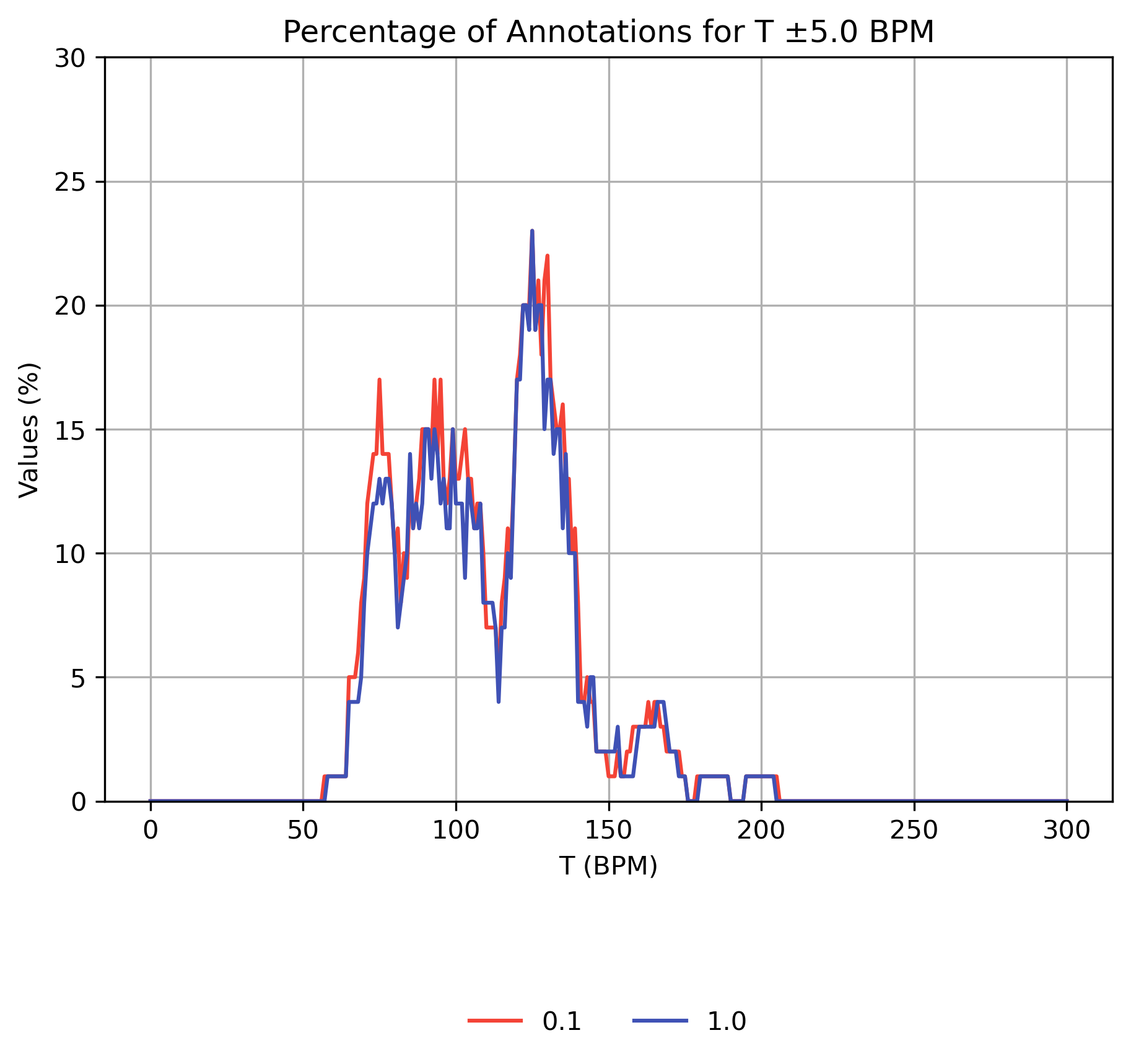
Smoothed Tempo Distribution
Figure 1: Percentage of values in tempo interval.
CSV JSON LATEX PICKLE SVG PDF PNG
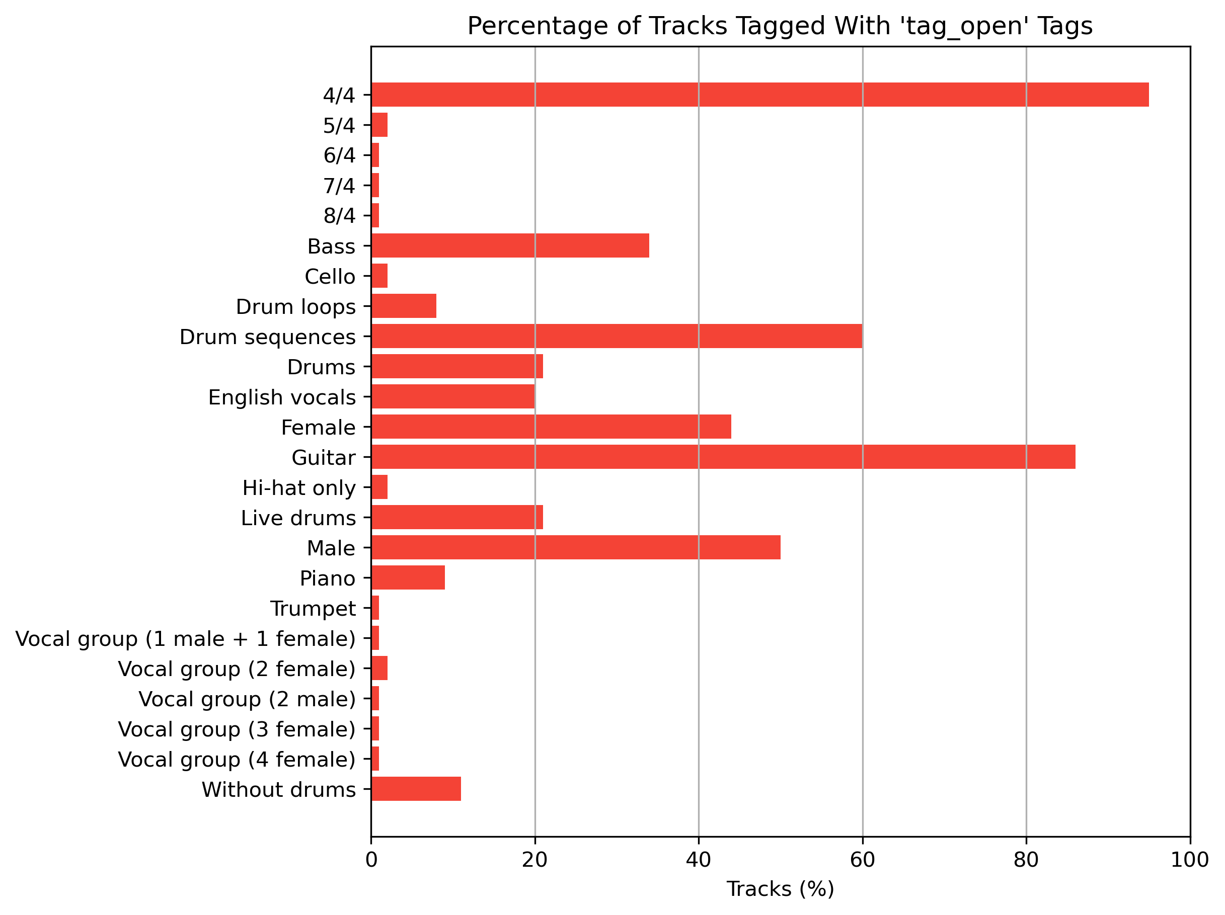
Tag Distribution for ‘tag_open’
Figure 2: Percentage of tracks tagged with tags from namespace ‘tag_open’. Annotations are from reference 1.0.
CSV JSON LATEX PICKLE SVG PDF PNG
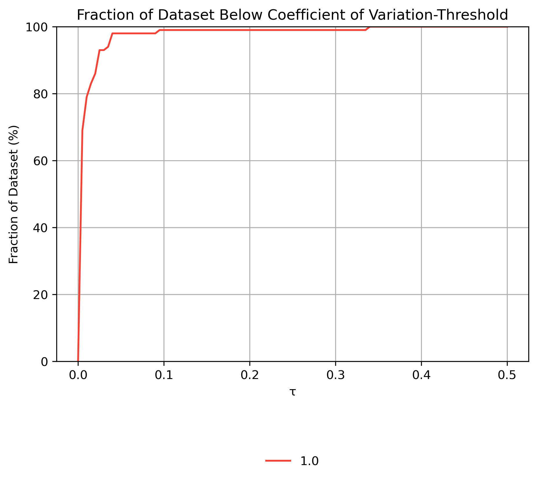
Beat-Based Tempo Variation
Figure 3: Fraction of the dataset with beat-annotated tracks with cvar < τ.
CSV JSON LATEX PICKLE SVG PDF PNG
Estimates for ‘rwc_mdb_p’
Estimators
boeck2015/tempodetector2016_default
| Attribute | Value |
|---|---|
| Corpus | rwc_mdb_p |
| Version | 0.17.dev0 |
| Annotation Tools | TempoDetector.2016, madmom, https://github.com/CPJKU/madmom |
| Annotator, bibtex | Boeck2015 |
davies2009/mirex_qm_tempotracker
| Attribute | Value | |
|---|---|---|
| Corpus | rwc_mdb_p | |
| Version | 1.0 | |
| Annotation Tools | QM Tempotracker, Sonic Annotator plugin. https://code.soundsoftware.ac.uk/projects/mirex2013/repository/show/audio_tempo_estimation/qm-tempotracker Note that the current macOS build of ‘qm-vamp-plugins’ was used. | |
| Annotator, bibtex | Davies2009 | Davies2007 |
percival2014/stem
| Attribute | Value |
|---|---|
| Corpus | rwc_mdb_p |
| Version | 1.0 |
| Annotation Tools | percival 2014, ‘tempo’ implementation from Marsyas, http://marsyas.info, git checkout tempo-stem |
| Annotator, bibtex | Percival2014 |
schreiber2014/default
| Attribute | Value |
|---|---|
| Corpus | rwc_mdb_p |
| Version | 0.0.1 |
| Annotation Tools | schreiber 2014, http://www.tagtraum.com/tempo_estimation.html |
| Annotator, bibtex | Schreiber2014 |
schreiber2017/ismir2017
| Attribute | Value |
|---|---|
| Corpus | rwc_mdb_p |
| Version | 0.0.4 |
| Annotation Tools | schreiber 2017, model=ismir2017, http://www.tagtraum.com/tempo_estimation.html |
| Annotator, bibtex | Schreiber2017 |
schreiber2017/mirex2017
| Attribute | Value |
|---|---|
| Corpus | rwc_mdb_p |
| Version | 0.0.4 |
| Annotation Tools | schreiber 2017, model=mirex2017, http://www.tagtraum.com/tempo_estimation.html |
| Annotator, bibtex | Schreiber2017 |
schreiber2018/cnn
| Attribute | Value |
|---|---|
| Corpus | |
| Version | 0.0.3 |
| Data Source | Hendrik Schreiber, Meinard Müller. A Single-Step Approach to Musical Tempo Estimation Using a Convolutional Neural Network. In Proceedings of the 19th International Society for Music Information Retrieval Conference (ISMIR), Paris, France, Sept. 2018. |
| Annotation Tools | schreiber tempo-cnn (model=cnn), https://github.com/hendriks73/tempo-cnn |
schreiber2018/fcn
| Attribute | Value |
|---|---|
| Corpus | |
| Version | 0.0.3 |
| Data Source | Hendrik Schreiber, Meinard Müller. A Single-Step Approach to Musical Tempo Estimation Using a Convolutional Neural Network. In Proceedings of the 19th International Society for Music Information Retrieval Conference (ISMIR), Paris, France, Sept. 2018. |
| Annotation Tools | schreiber tempo-cnn (model=fcn), https://github.com/hendriks73/tempo-cnn |
schreiber2018/ismir2018
| Attribute | Value |
|---|---|
| Corpus | |
| Version | 0.0.3 |
| Data Source | Hendrik Schreiber, Meinard Müller. A Single-Step Approach to Musical Tempo Estimation Using a Convolutional Neural Network. In Proceedings of the 19th International Society for Music Information Retrieval Conference (ISMIR), Paris, France, Sept. 2018. |
| Annotation Tools | schreiber tempo-cnn (model=ismir2018), https://github.com/hendriks73/tempo-cnn |
Basic Statistics
| Estimator | Size | Min | Max | Avg | Stdev | Sweet Oct. Start | Sweet Oct. Coverage |
|---|---|---|---|---|---|---|---|
| boeck2015/tempodetector2016_default | 100 | 41.96 | 187.50 | 90.99 | 31.62 | 54.00 | 0.67 |
| davies2009/mirex_qm_tempotracker | 100 | 80.75 | 178.21 | 123.00 | 24.28 | 87.00 | 0.95 |
| percival2014/stem | 100 | 60.09 | 148.72 | 102.91 | 22.33 | 70.00 | 0.94 |
| schreiber2014/default | 100 | 59.93 | 157.99 | 101.33 | 22.55 | 68.00 | 0.92 |
| schreiber2017/ismir2017 | 100 | 54.00 | 163.00 | 106.23 | 24.79 | 69.00 | 0.90 |
| schreiber2017/mirex2017 | 100 | 60.01 | 163.00 | 107.34 | 23.65 | 69.00 | 0.92 |
| schreiber2018/cnn | 100 | 60.00 | 188.00 | 113.65 | 29.37 | 70.00 | 0.85 |
| schreiber2018/fcn | 100 | 54.00 | 197.00 | 109.32 | 29.51 | 70.00 | 0.87 |
| schreiber2018/ismir2018 | 100 | 70.00 | 188.00 | 110.28 | 24.17 | 71.00 | 0.92 |
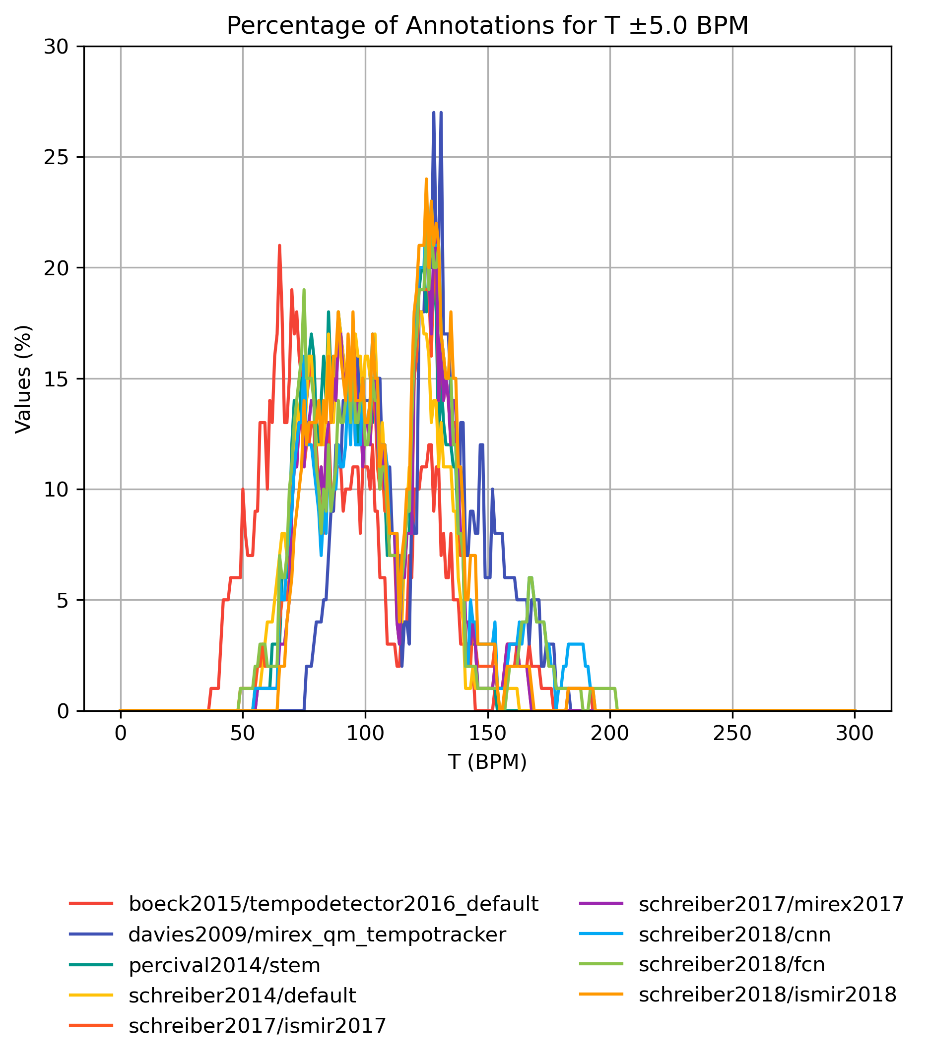
Smoothed Tempo Distribution
Figure 4: Percentage of values in tempo interval.
CSV JSON LATEX PICKLE SVG PDF PNG
Accuracy
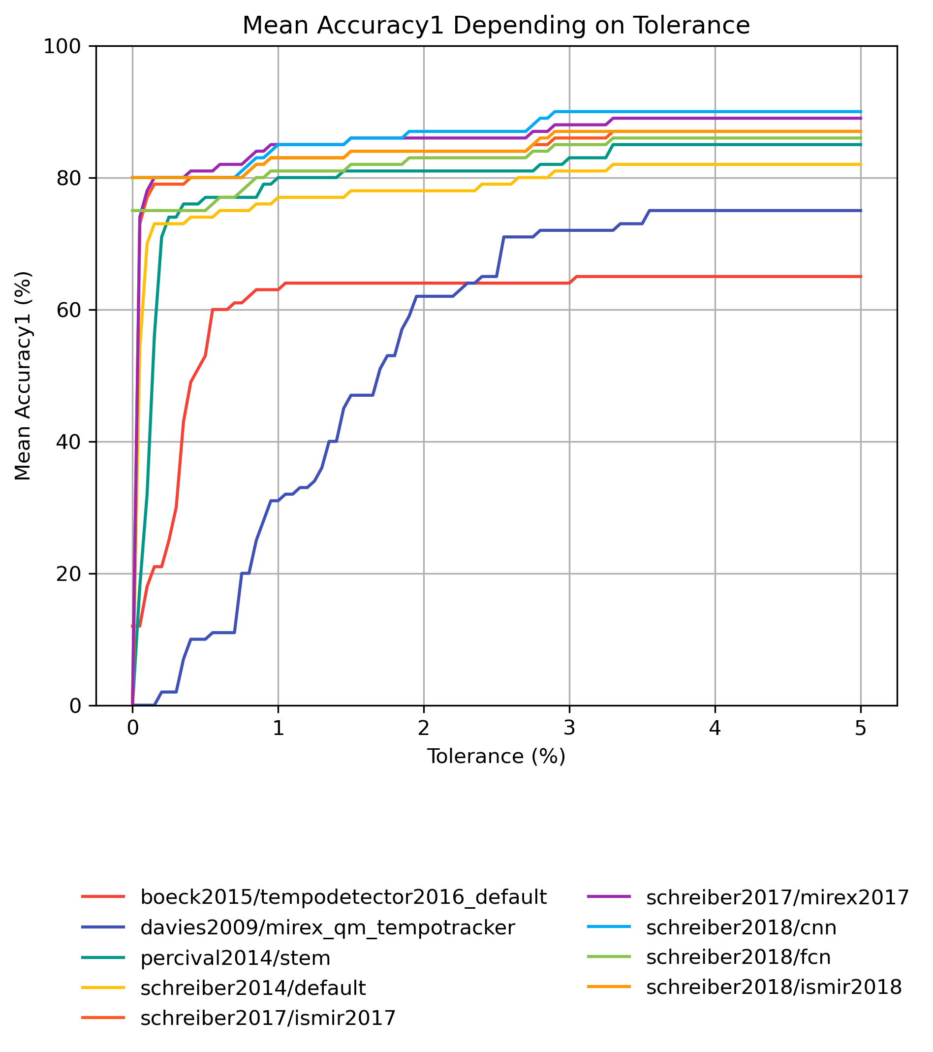
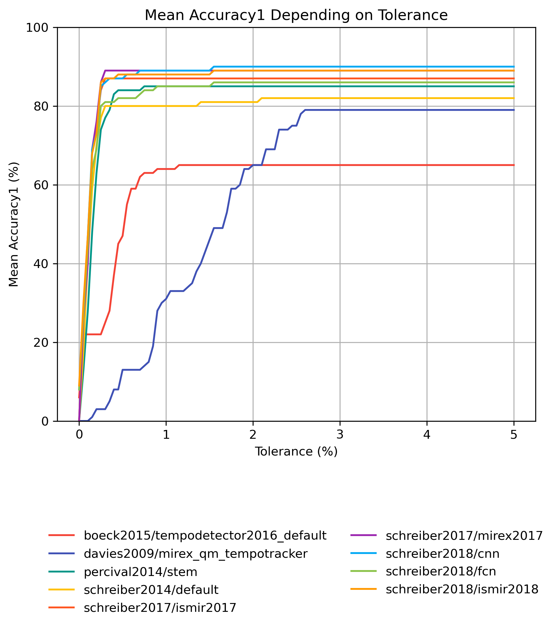
Accuracy1 is defined as the percentage of correct estimates, allowing a 4% tolerance for individual BPM values.
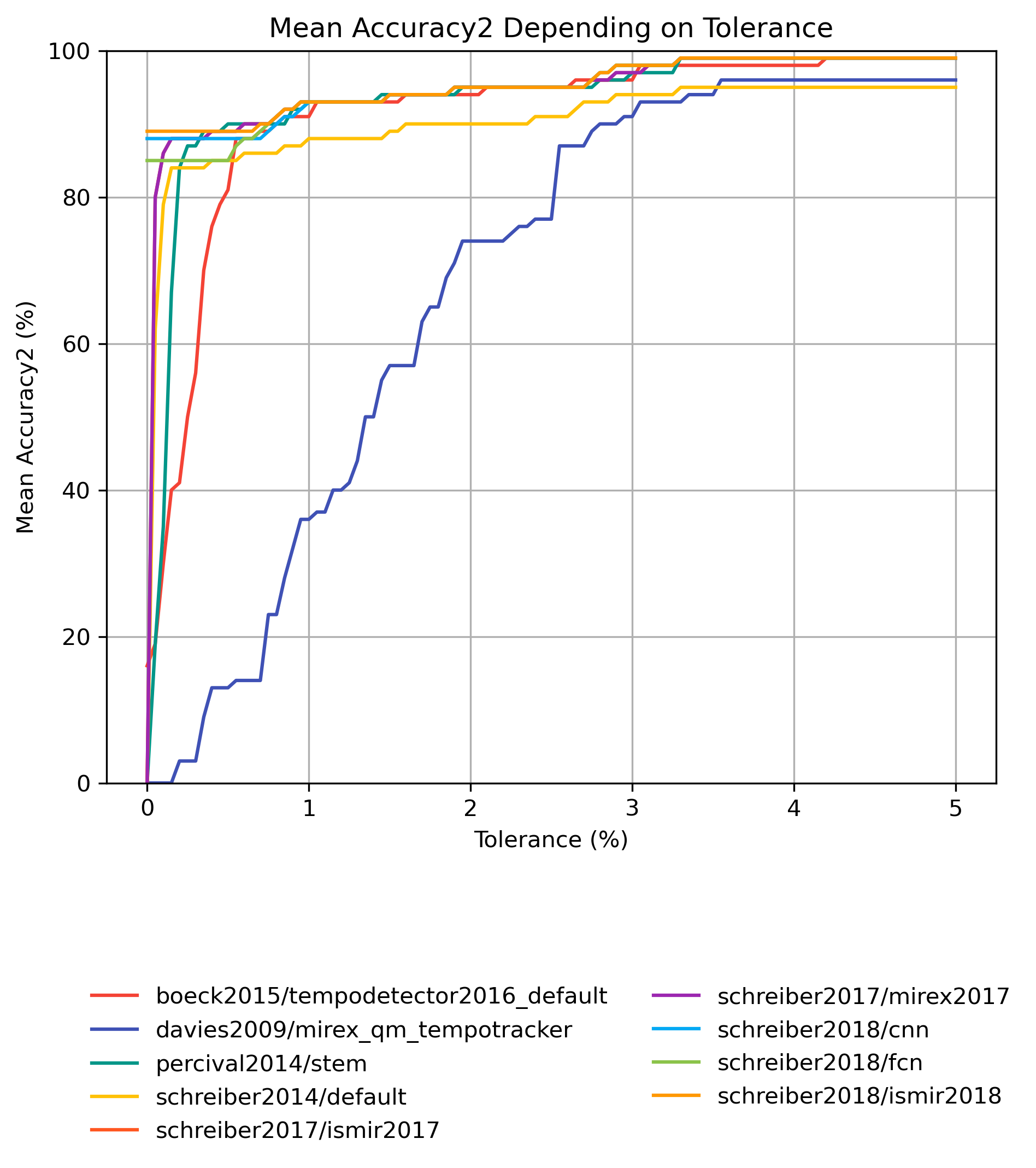
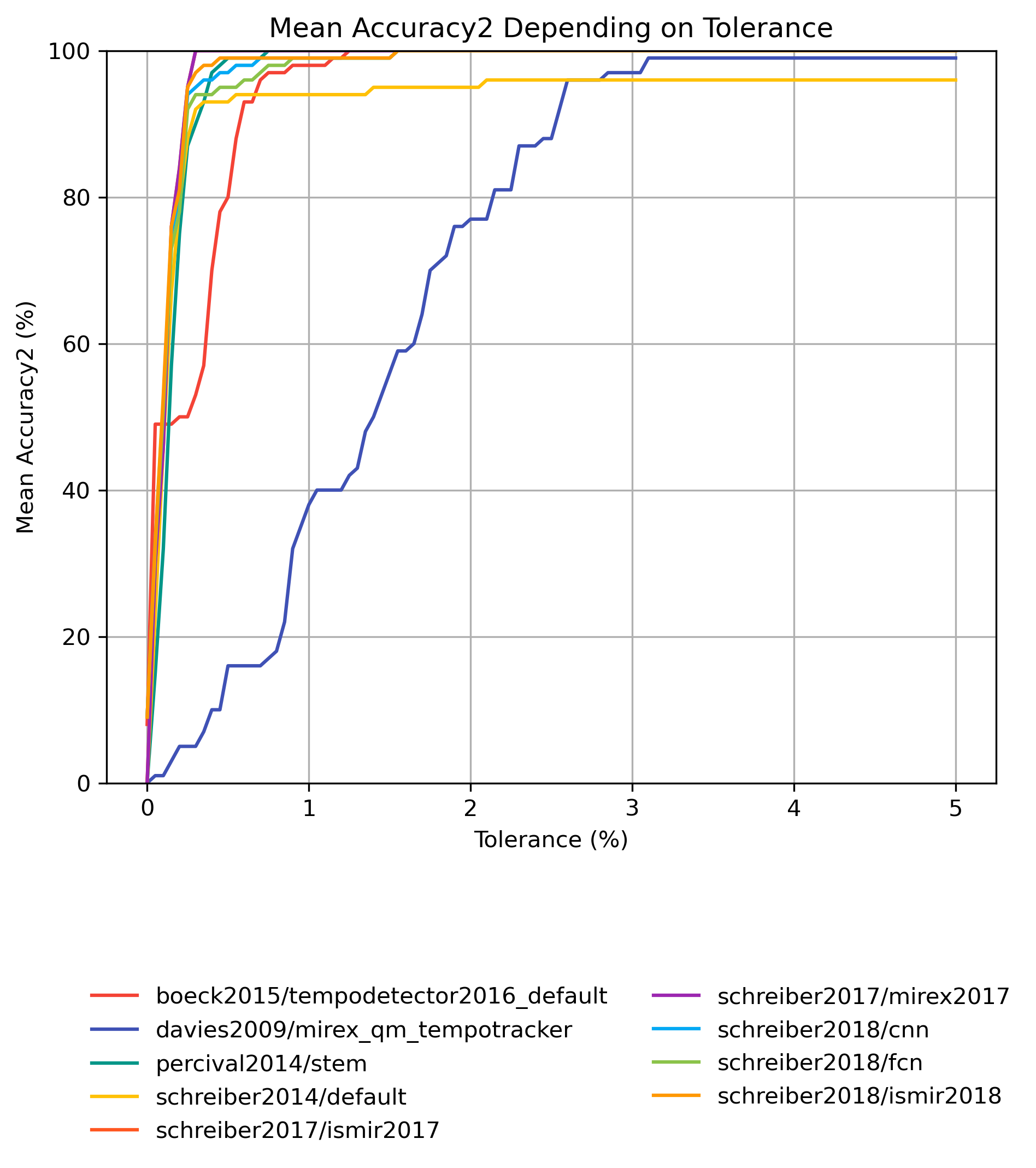
Accuracy2 additionally permits estimates to be wrong by a factor of 2, 3, 1/2 or 1/3 (so-called octave errors).
See [Gouyon2006].
Note: When comparing accuracy values for different algorithms, keep in mind that an algorithm may have been trained on the test set or that the test set may have even been created using one of the tested algorithms.
Accuracy Results for 0.1
| Estimator | Accuracy1 | Accuracy2 |
|---|---|---|
| schreiber2018/cnn | 0.9000 | 0.9900 |
| schreiber2017/mirex2017 | 0.8900 | 0.9900 |
| schreiber2018/ismir2018 | 0.8700 | 0.9900 |
| schreiber2017/ismir2017 | 0.8700 | 0.9900 |
| schreiber2018/fcn | 0.8600 | 0.9900 |
| percival2014/stem | 0.8500 | 0.9900 |
| schreiber2014/default | 0.8200 | 0.9500 |
| davies2009/mirex_qm_tempotracker | 0.7500 | 0.9600 |
| boeck2015/tempodetector2016_default | 0.6500 | 0.9800 |
Table 3: Mean accuracy of estimates compared to version 0.1 with 4% tolerance ordered by Accuracy1.
Raw data Accuracy1: CSV JSON LATEX PICKLE
Raw data Accuracy2: CSV JSON LATEX PICKLE
Accuracy1 for 0.1
Figure 5: Mean Accuracy1 for estimates compared to version 0.1 depending on tolerance.
CSV JSON LATEX PICKLE SVG PDF PNG
Accuracy2 for 0.1
Figure 6: Mean Accuracy2 for estimates compared to version 0.1 depending on tolerance.
CSV JSON LATEX PICKLE SVG PDF PNG
Accuracy Results for 1.0
| Estimator | Accuracy1 | Accuracy2 |
|---|---|---|
| schreiber2018/cnn | 0.9000 | 1.0000 |
| schreiber2018/ismir2018 | 0.8900 | 1.0000 |
| schreiber2017/mirex2017 | 0.8900 | 1.0000 |
| schreiber2017/ismir2017 | 0.8700 | 1.0000 |
| schreiber2018/fcn | 0.8600 | 1.0000 |
| percival2014/stem | 0.8500 | 1.0000 |
| schreiber2014/default | 0.8200 | 0.9600 |
| davies2009/mirex_qm_tempotracker | 0.7900 | 0.9900 |
| boeck2015/tempodetector2016_default | 0.6500 | 1.0000 |
Table 4: Mean accuracy of estimates compared to version 1.0 with 4% tolerance ordered by Accuracy1.
Raw data Accuracy1: CSV JSON LATEX PICKLE
Raw data Accuracy2: CSV JSON LATEX PICKLE
Accuracy1 for 1.0
Figure 7: Mean Accuracy1 for estimates compared to version 1.0 depending on tolerance.
CSV JSON LATEX PICKLE SVG PDF PNG
Accuracy2 for 1.0
Figure 8: Mean Accuracy2 for estimates compared to version 1.0 depending on tolerance.
CSV JSON LATEX PICKLE SVG PDF PNG
Differing Items
For which items did a given estimator not estimate a correct value with respect to a given ground truth? Are there items which are either very difficult, not suitable for the task, or incorrectly annotated and therefore never estimated correctly, regardless which estimator is used?
Differing Items Accuracy1
Items with different tempo annotations (Accuracy1, 4% tolerance) in different versions:
0.1 compared with boeck2015/tempodetector2016_default (35 differences): ‘RM-P001’ ‘RM-P003’ ‘RM-P005’ ‘RM-P010’ ‘RM-P012’ ‘RM-P015’ ‘RM-P018’ ‘RM-P020’ ‘RM-P022’ ‘RM-P023’ ‘RM-P027’ … CSV
0.1 compared with davies2009/mirex_qm_tempotracker (25 differences): ‘RM-P004’ ‘RM-P009’ ‘RM-P037’ ‘RM-P039’ ‘RM-P041’ ‘RM-P045’ ‘RM-P046’ ‘RM-P055’ ‘RM-P056’ ‘RM-P057’ ‘RM-P060’ … CSV
0.1 compared with percival2014/stem (15 differences): ‘RM-P009’ ‘RM-P026’ ‘RM-P035’ ‘RM-P037’ ‘RM-P041’ ‘RM-P043’ ‘RM-P046’ ‘RM-P053’ ‘RM-P060’ ‘RM-P069’ ‘RM-P072’ … CSV
0.1 compared with schreiber2014/default (18 differences): ‘RM-P001’ ‘RM-P009’ ‘RM-P031’ ‘RM-P035’ ‘RM-P037’ ‘RM-P038’ ‘RM-P041’ ‘RM-P043’ ‘RM-P046’ ‘RM-P053’ ‘RM-P057’ … CSV
0.1 compared with schreiber2017/ismir2017 (13 differences): ‘RM-P035’ ‘RM-P037’ ‘RM-P041’ ‘RM-P046’ ‘RM-P056’ ‘RM-P057’ ‘RM-P062’ ‘RM-P072’ ‘RM-P073’ ‘RM-P075’ ‘RM-P077’ … CSV
0.1 compared with schreiber2017/mirex2017 (11 differences): ‘RM-P035’ ‘RM-P037’ ‘RM-P041’ ‘RM-P046’ ‘RM-P057’ ‘RM-P062’ ‘RM-P069’ ‘RM-P072’ ‘RM-P073’ ‘RM-P077’ ‘RM-P095’ … CSV
0.1 compared with schreiber2018/cnn (10 differences): ‘RM-P004’ ‘RM-P034’ ‘RM-P041’ ‘RM-P048’ ‘RM-P056’ ‘RM-P069’ ‘RM-P072’ ‘RM-P077’ ‘RM-P083’ ‘RM-P097’ CSV
0.1 compared with schreiber2018/fcn (14 differences): ‘RM-P004’ ‘RM-P026’ ‘RM-P027’ ‘RM-P041’ ‘RM-P048’ ‘RM-P056’ ‘RM-P060’ ‘RM-P069’ ‘RM-P072’ ‘RM-P073’ ‘RM-P075’ … CSV
0.1 compared with schreiber2018/ismir2018 (13 differences): ‘RM-P009’ ‘RM-P026’ ‘RM-P035’ ‘RM-P037’ ‘RM-P041’ ‘RM-P046’ ‘RM-P056’ ‘RM-P062’ ‘RM-P069’ ‘RM-P071’ ‘RM-P072’ … CSV
1.0 compared with boeck2015/tempodetector2016_default (35 differences): ‘RM-P001’ ‘RM-P003’ ‘RM-P005’ ‘RM-P010’ ‘RM-P012’ ‘RM-P015’ ‘RM-P018’ ‘RM-P020’ ‘RM-P022’ ‘RM-P023’ ‘RM-P027’ … CSV
1.0 compared with davies2009/mirex_qm_tempotracker (21 differences): ‘RM-P004’ ‘RM-P009’ ‘RM-P037’ ‘RM-P039’ ‘RM-P041’ ‘RM-P045’ ‘RM-P046’ ‘RM-P055’ ‘RM-P056’ ‘RM-P057’ ‘RM-P060’ … CSV
1.0 compared with percival2014/stem (15 differences): ‘RM-P009’ ‘RM-P026’ ‘RM-P035’ ‘RM-P037’ ‘RM-P041’ ‘RM-P043’ ‘RM-P046’ ‘RM-P053’ ‘RM-P060’ ‘RM-P069’ ‘RM-P071’ … CSV
1.0 compared with schreiber2014/default (18 differences): ‘RM-P001’ ‘RM-P009’ ‘RM-P031’ ‘RM-P035’ ‘RM-P037’ ‘RM-P038’ ‘RM-P041’ ‘RM-P043’ ‘RM-P046’ ‘RM-P053’ ‘RM-P057’ … CSV
1.0 compared with schreiber2017/ismir2017 (13 differences): ‘RM-P035’ ‘RM-P037’ ‘RM-P041’ ‘RM-P046’ ‘RM-P056’ ‘RM-P057’ ‘RM-P062’ ‘RM-P071’ ‘RM-P073’ ‘RM-P075’ ‘RM-P077’ … CSV
1.0 compared with schreiber2017/mirex2017 (11 differences): ‘RM-P035’ ‘RM-P037’ ‘RM-P041’ ‘RM-P046’ ‘RM-P057’ ‘RM-P062’ ‘RM-P069’ ‘RM-P071’ ‘RM-P073’ ‘RM-P077’ ‘RM-P095’ … CSV
1.0 compared with schreiber2018/cnn (10 differences): ‘RM-P004’ ‘RM-P034’ ‘RM-P041’ ‘RM-P048’ ‘RM-P056’ ‘RM-P069’ ‘RM-P071’ ‘RM-P077’ ‘RM-P083’ ‘RM-P097’ CSV
1.0 compared with schreiber2018/fcn (14 differences): ‘RM-P004’ ‘RM-P026’ ‘RM-P027’ ‘RM-P041’ ‘RM-P048’ ‘RM-P056’ ‘RM-P060’ ‘RM-P069’ ‘RM-P071’ ‘RM-P073’ ‘RM-P075’ … CSV
1.0 compared with schreiber2018/ismir2018 (11 differences): ‘RM-P009’ ‘RM-P026’ ‘RM-P035’ ‘RM-P037’ ‘RM-P041’ ‘RM-P046’ ‘RM-P056’ ‘RM-P062’ ‘RM-P069’ ‘RM-P095’ ‘RM-P097’ … CSV
None of the estimators estimated the following item ‘correctly’ using Accuracy1: ‘RM-P041’ CSV
Differing Items Accuracy2
Items with different tempo annotations (Accuracy2, 4% tolerance) in different versions:
0.1 compared with boeck2015/tempodetector2016_default (2 differences): ‘RM-P072’ ‘RM-P073’ CSV
0.1 compared with davies2009/mirex_qm_tempotracker (4 differences): ‘RM-P060’ ‘RM-P072’ ‘RM-P073’ ‘RM-P097’ CSV
0.1 compared with percival2014/stem (1 differences): ‘RM-P072’ CSV
0.1 compared with schreiber2014/default (5 differences): ‘RM-P009’ ‘RM-P038’ ‘RM-P053’ ‘RM-P057’ ‘RM-P072’ CSV
0.1 compared with schreiber2017/ismir2017 (1 differences): ‘RM-P072’ CSV
0.1 compared with schreiber2017/mirex2017 (1 differences): ‘RM-P072’ CSV
0.1 compared with schreiber2018/cnn (1 differences): ‘RM-P072’ CSV
0.1 compared with schreiber2018/fcn (1 differences): ‘RM-P072’ CSV
0.1 compared with schreiber2018/ismir2018 (1 differences): ‘RM-P072’ CSV
1.0 compared with boeck2015/tempodetector2016_default: No differences.
1.0 compared with davies2009/mirex_qm_tempotracker (1 differences): ‘RM-P060’ CSV
1.0 compared with percival2014/stem: No differences.
1.0 compared with schreiber2014/default (4 differences): ‘RM-P009’ ‘RM-P038’ ‘RM-P053’ ‘RM-P057’ CSV
1.0 compared with schreiber2017/ismir2017: No differences.
1.0 compared with schreiber2017/mirex2017: No differences.
1.0 compared with schreiber2018/cnn: No differences.
1.0 compared with schreiber2018/fcn: No differences.
1.0 compared with schreiber2018/ismir2018: No differences.
All tracks were estimated ‘correctly’ by at least one system.
Significance of Differences
| Estimator | boeck2015/tempodetector2016_default | davies2009/mirex_qm_tempotracker | percival2014/stem | schreiber2014/default | schreiber2017/ismir2017 | schreiber2017/mirex2017 | schreiber2018/cnn | schreiber2018/fcn | schreiber2018/ismir2018 |
|---|---|---|---|---|---|---|---|---|---|
| boeck2015/tempodetector2016_default | 1.0000 | 0.0649 | 0.0012 | 0.0033 | 0.0002 | 0.0000 | 0.0000 | 0.0005 | 0.0001 |
| davies2009/mirex_qm_tempotracker | 0.0649 | 1.0000 | 0.3075 | 0.7111 | 0.1338 | 0.0414 | 0.0347 | 0.2295 | 0.0309 |
| percival2014/stem | 0.0012 | 0.3075 | 1.0000 | 0.5488 | 0.7744 | 0.3437 | 0.3018 | 1.0000 | 0.3437 |
| schreiber2014/default | 0.0033 | 0.7111 | 0.5488 | 1.0000 | 0.2266 | 0.0654 | 0.1153 | 0.5235 | 0.1435 |
| schreiber2017/ismir2017 | 0.0002 | 0.1338 | 0.7744 | 0.2266 | 1.0000 | 0.6250 | 0.5811 | 1.0000 | 0.7539 |
| schreiber2017/mirex2017 | 0.0000 | 0.0414 | 0.3437 | 0.0654 | 0.6250 | 1.0000 | 1.0000 | 0.6072 | 1.0000 |
| schreiber2018/cnn | 0.0000 | 0.0347 | 0.3018 | 0.1153 | 0.5811 | 1.0000 | 1.0000 | 0.2891 | 1.0000 |
| schreiber2018/fcn | 0.0005 | 0.2295 | 1.0000 | 0.5235 | 1.0000 | 0.6072 | 0.2891 | 1.0000 | 0.6291 |
| schreiber2018/ismir2018 | 0.0001 | 0.0309 | 0.3437 | 0.1435 | 0.7539 | 1.0000 | 1.0000 | 0.6291 | 1.0000 |
Table 5: McNemar p-values, using reference annotations 1.0 as groundtruth with Accuracy1 [Gouyon2006]. H0: both estimators disagree with the groundtruth to the same amount. If p<=ɑ, reject H0, i.e. we have a significant difference in the disagreement with the groundtruth. In the table, p-values<0.05 are set in bold.
| Estimator | boeck2015/tempodetector2016_default | davies2009/mirex_qm_tempotracker | percival2014/stem | schreiber2014/default | schreiber2017/ismir2017 | schreiber2017/mirex2017 | schreiber2018/cnn | schreiber2018/fcn | schreiber2018/ismir2018 |
|---|---|---|---|---|---|---|---|---|---|
| boeck2015/tempodetector2016_default | 1.0000 | 0.1934 | 0.0012 | 0.0033 | 0.0002 | 0.0000 | 0.0000 | 0.0005 | 0.0005 |
| davies2009/mirex_qm_tempotracker | 0.1934 | 1.0000 | 0.0755 | 0.2649 | 0.0169 | 0.0026 | 0.0026 | 0.0433 | 0.0075 |
| percival2014/stem | 0.0012 | 0.0755 | 1.0000 | 0.5488 | 0.7744 | 0.3437 | 0.3018 | 1.0000 | 0.7539 |
| schreiber2014/default | 0.0033 | 0.2649 | 0.5488 | 1.0000 | 0.2266 | 0.0654 | 0.1153 | 0.5235 | 0.3323 |
| schreiber2017/ismir2017 | 0.0002 | 0.0169 | 0.7744 | 0.2266 | 1.0000 | 0.6250 | 0.5811 | 1.0000 | 1.0000 |
| schreiber2017/mirex2017 | 0.0000 | 0.0026 | 0.3437 | 0.0654 | 0.6250 | 1.0000 | 1.0000 | 0.6072 | 0.7266 |
| schreiber2018/cnn | 0.0000 | 0.0026 | 0.3018 | 0.1153 | 0.5811 | 1.0000 | 1.0000 | 0.2891 | 0.5811 |
| schreiber2018/fcn | 0.0005 | 0.0433 | 1.0000 | 0.5235 | 1.0000 | 0.6072 | 0.2891 | 1.0000 | 1.0000 |
| schreiber2018/ismir2018 | 0.0005 | 0.0075 | 0.7539 | 0.3323 | 1.0000 | 0.7266 | 0.5811 | 1.0000 | 1.0000 |
Table 6: McNemar p-values, using reference annotations 0.1 as groundtruth with Accuracy1 [Gouyon2006]. H0: both estimators disagree with the groundtruth to the same amount. If p<=ɑ, reject H0, i.e. we have a significant difference in the disagreement with the groundtruth. In the table, p-values<0.05 are set in bold.
| Estimator | boeck2015/tempodetector2016_default | davies2009/mirex_qm_tempotracker | percival2014/stem | schreiber2014/default | schreiber2017/ismir2017 | schreiber2017/mirex2017 | schreiber2018/cnn | schreiber2018/fcn | schreiber2018/ismir2018 |
|---|---|---|---|---|---|---|---|---|---|
| boeck2015/tempodetector2016_default | 1.0000 | 1.0000 | 1.0000 | 0.1250 | 1.0000 | 1.0000 | 1.0000 | 1.0000 | 1.0000 |
| davies2009/mirex_qm_tempotracker | 1.0000 | 1.0000 | 1.0000 | 0.3750 | 1.0000 | 1.0000 | 1.0000 | 1.0000 | 1.0000 |
| percival2014/stem | 1.0000 | 1.0000 | 1.0000 | 0.1250 | 1.0000 | 1.0000 | 1.0000 | 1.0000 | 1.0000 |
| schreiber2014/default | 0.1250 | 0.3750 | 0.1250 | 1.0000 | 0.1250 | 0.1250 | 0.1250 | 0.1250 | 0.1250 |
| schreiber2017/ismir2017 | 1.0000 | 1.0000 | 1.0000 | 0.1250 | 1.0000 | 1.0000 | 1.0000 | 1.0000 | 1.0000 |
| schreiber2017/mirex2017 | 1.0000 | 1.0000 | 1.0000 | 0.1250 | 1.0000 | 1.0000 | 1.0000 | 1.0000 | 1.0000 |
| schreiber2018/cnn | 1.0000 | 1.0000 | 1.0000 | 0.1250 | 1.0000 | 1.0000 | 1.0000 | 1.0000 | 1.0000 |
| schreiber2018/fcn | 1.0000 | 1.0000 | 1.0000 | 0.1250 | 1.0000 | 1.0000 | 1.0000 | 1.0000 | 1.0000 |
| schreiber2018/ismir2018 | 1.0000 | 1.0000 | 1.0000 | 0.1250 | 1.0000 | 1.0000 | 1.0000 | 1.0000 | 1.0000 |
Table 7: McNemar p-values, using reference annotations 1.0 as groundtruth with Accuracy2 [Gouyon2006]. H0: both estimators disagree with the groundtruth to the same amount. If p<=ɑ, reject H0, i.e. we have a significant difference in the disagreement with the groundtruth. In the table, p-values<0.05 are set in bold.
| Estimator | boeck2015/tempodetector2016_default | davies2009/mirex_qm_tempotracker | percival2014/stem | schreiber2014/default | schreiber2017/ismir2017 | schreiber2017/mirex2017 | schreiber2018/cnn | schreiber2018/fcn | schreiber2018/ismir2018 |
|---|---|---|---|---|---|---|---|---|---|
| boeck2015/tempodetector2016_default | 1.0000 | 0.5000 | 1.0000 | 0.3750 | 1.0000 | 1.0000 | 1.0000 | 1.0000 | 1.0000 |
| davies2009/mirex_qm_tempotracker | 0.5000 | 1.0000 | 0.2500 | 1.0000 | 0.2500 | 0.2500 | 0.2500 | 0.2500 | 0.2500 |
| percival2014/stem | 1.0000 | 0.2500 | 1.0000 | 0.1250 | 1.0000 | 1.0000 | 1.0000 | 1.0000 | 1.0000 |
| schreiber2014/default | 0.3750 | 1.0000 | 0.1250 | 1.0000 | 0.1250 | 0.1250 | 0.1250 | 0.1250 | 0.1250 |
| schreiber2017/ismir2017 | 1.0000 | 0.2500 | 1.0000 | 0.1250 | 1.0000 | 1.0000 | 1.0000 | 1.0000 | 1.0000 |
| schreiber2017/mirex2017 | 1.0000 | 0.2500 | 1.0000 | 0.1250 | 1.0000 | 1.0000 | 1.0000 | 1.0000 | 1.0000 |
| schreiber2018/cnn | 1.0000 | 0.2500 | 1.0000 | 0.1250 | 1.0000 | 1.0000 | 1.0000 | 1.0000 | 1.0000 |
| schreiber2018/fcn | 1.0000 | 0.2500 | 1.0000 | 0.1250 | 1.0000 | 1.0000 | 1.0000 | 1.0000 | 1.0000 |
| schreiber2018/ismir2018 | 1.0000 | 0.2500 | 1.0000 | 0.1250 | 1.0000 | 1.0000 | 1.0000 | 1.0000 | 1.0000 |
Table 8: McNemar p-values, using reference annotations 0.1 as groundtruth with Accuracy2 [Gouyon2006]. H0: both estimators disagree with the groundtruth to the same amount. If p<=ɑ, reject H0, i.e. we have a significant difference in the disagreement with the groundtruth. In the table, p-values<0.05 are set in bold.
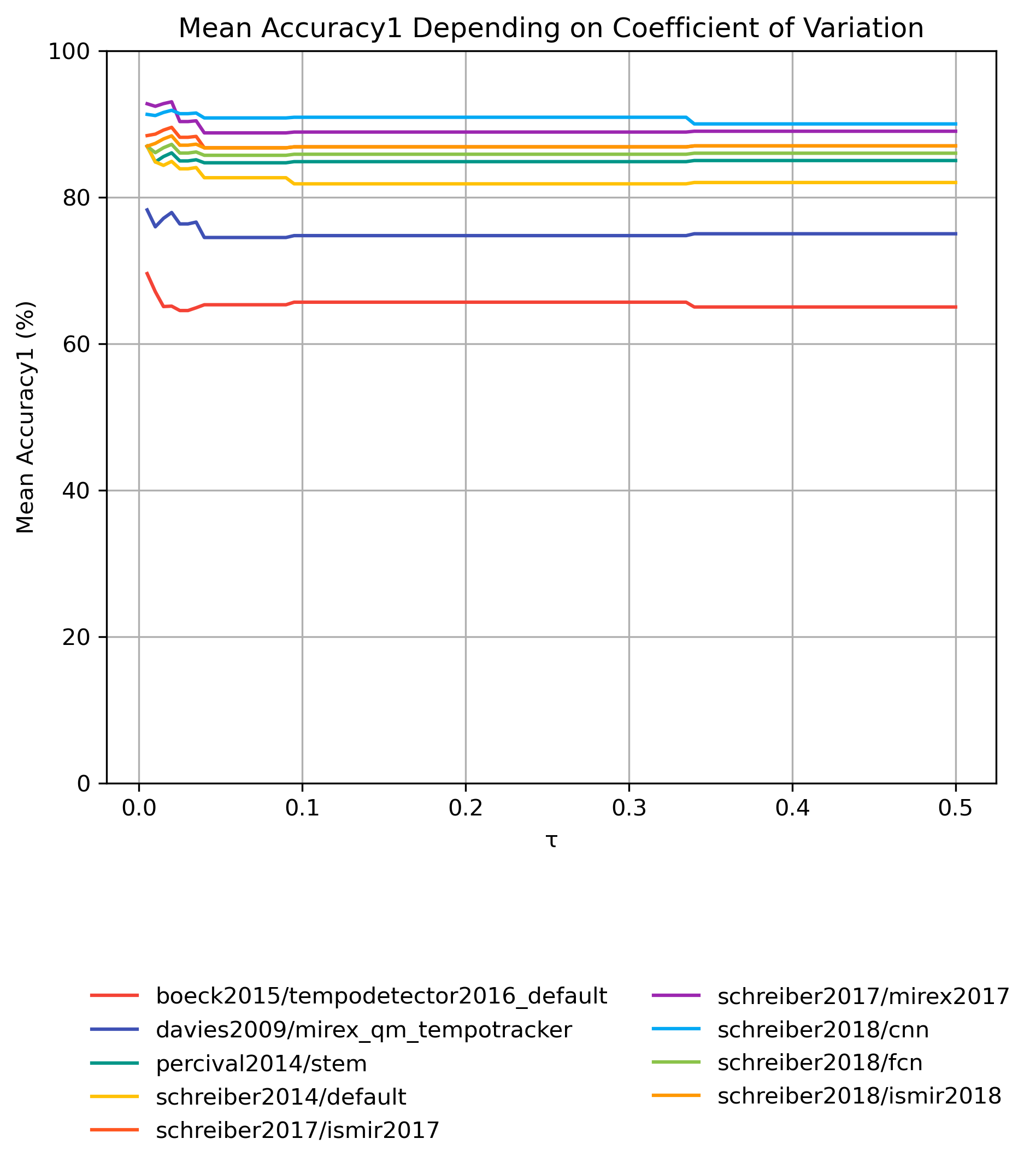
Accuracy1 on cvar-Subsets
How well does an estimator perform, when only taking tracks into account that have a cvar-value of less than τ, i.e., have a more or less stable beat?
Accuracy1 on cvar-Subsets for 0.1 based on cvar-Values from 1.0
Figure 9: Mean Accuracy1 compared to version 0.1 for tracks with cvar < τ based on beat annotations from 0.1.
CSV JSON LATEX PICKLE SVG PDF PNG
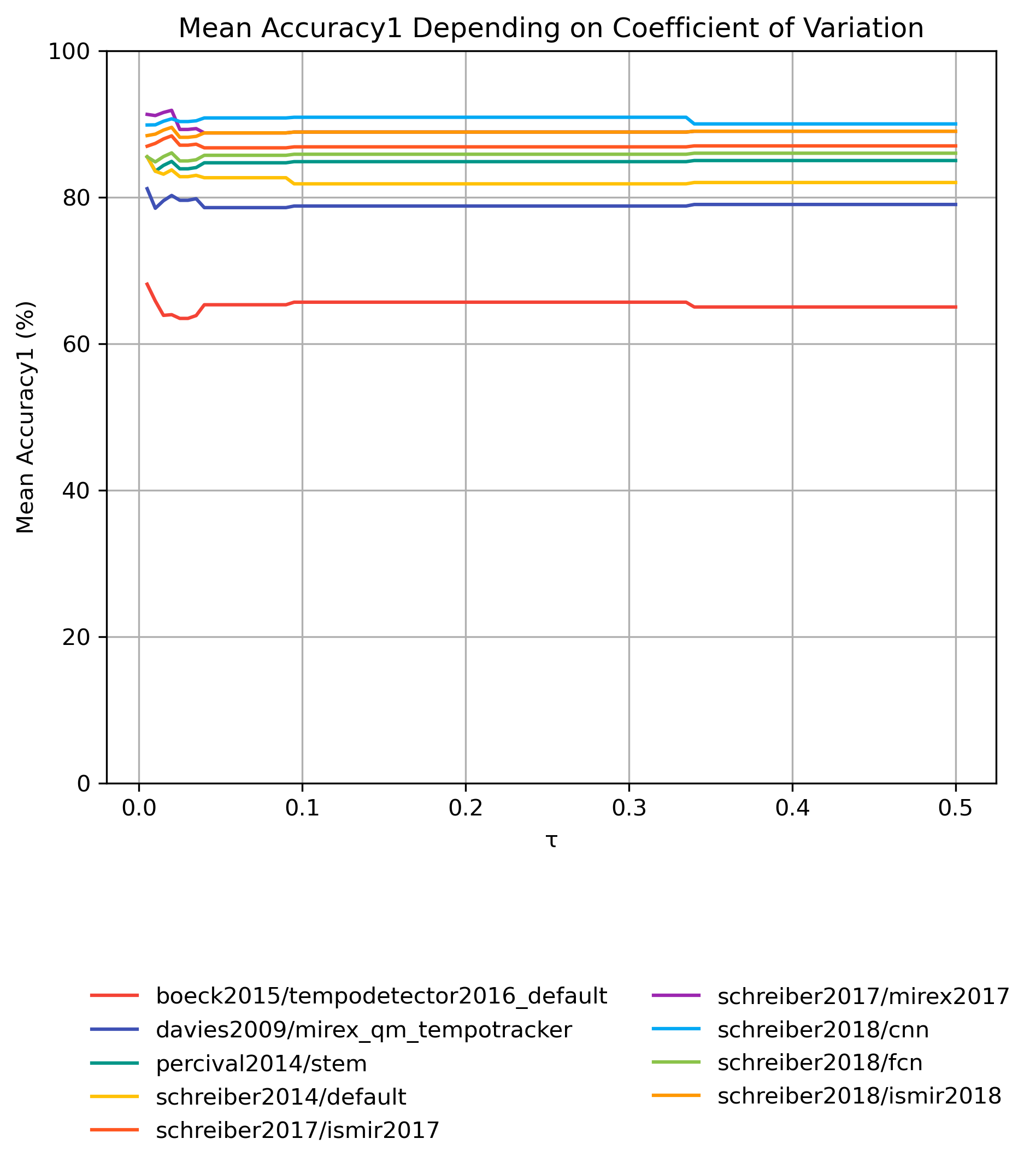
Accuracy1 on cvar-Subsets for 1.0 based on cvar-Values from 1.0
Figure 10: Mean Accuracy1 compared to version 1.0 for tracks with cvar < τ based on beat annotations from 1.0.
CSV JSON LATEX PICKLE SVG PDF PNG
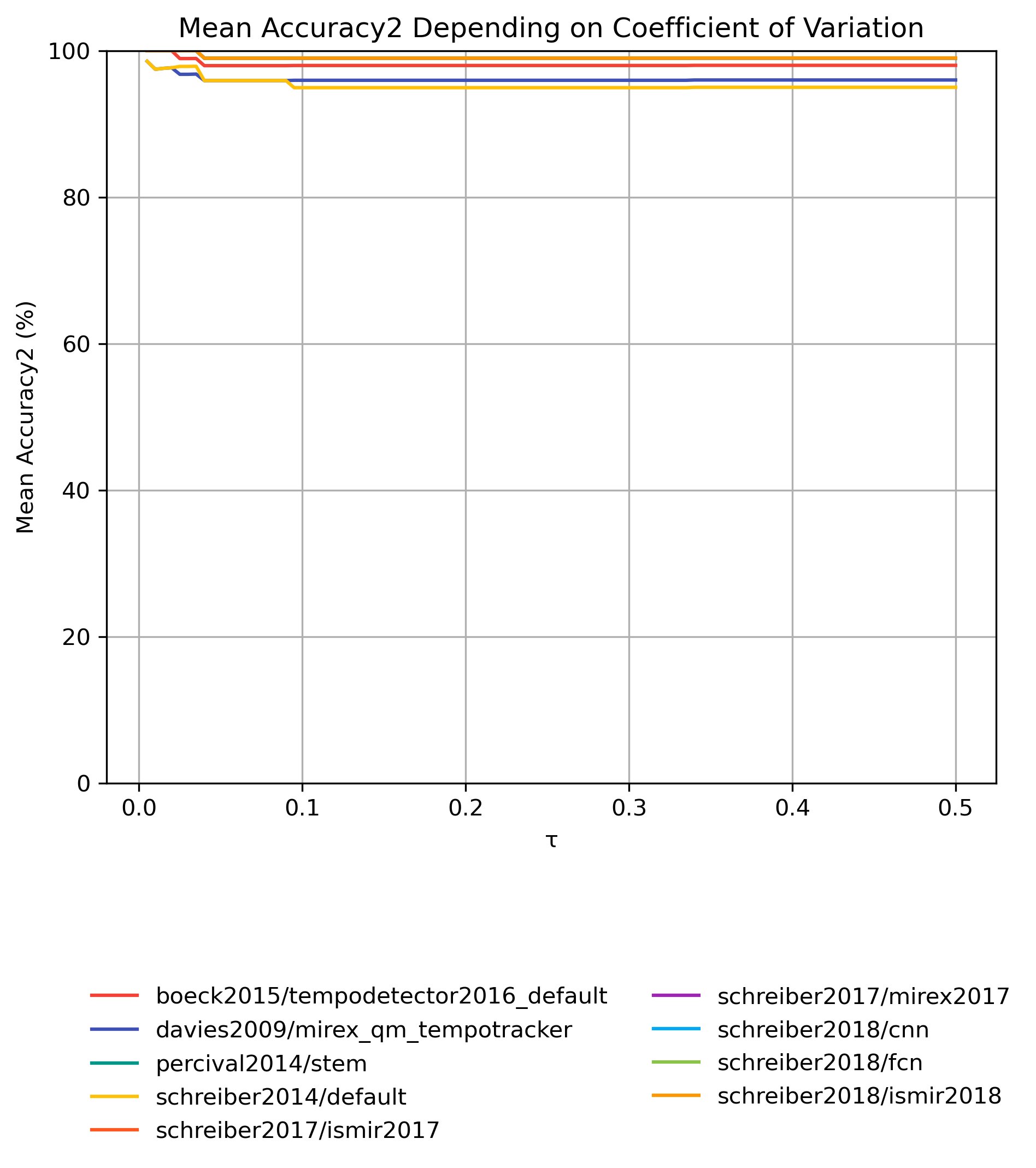
Accuracy2 on cvar-Subsets
How well does an estimator perform, when only taking tracks into account that have a cvar-value of less than τ, i.e., have a more or less stable beat?
Accuracy2 on cvar-Subsets for 0.1 based on cvar-Values from 1.0
Figure 11: Mean Accuracy2 compared to version 0.1 for tracks with cvar < τ based on beat annotations from 0.1.
CSV JSON LATEX PICKLE SVG PDF PNG
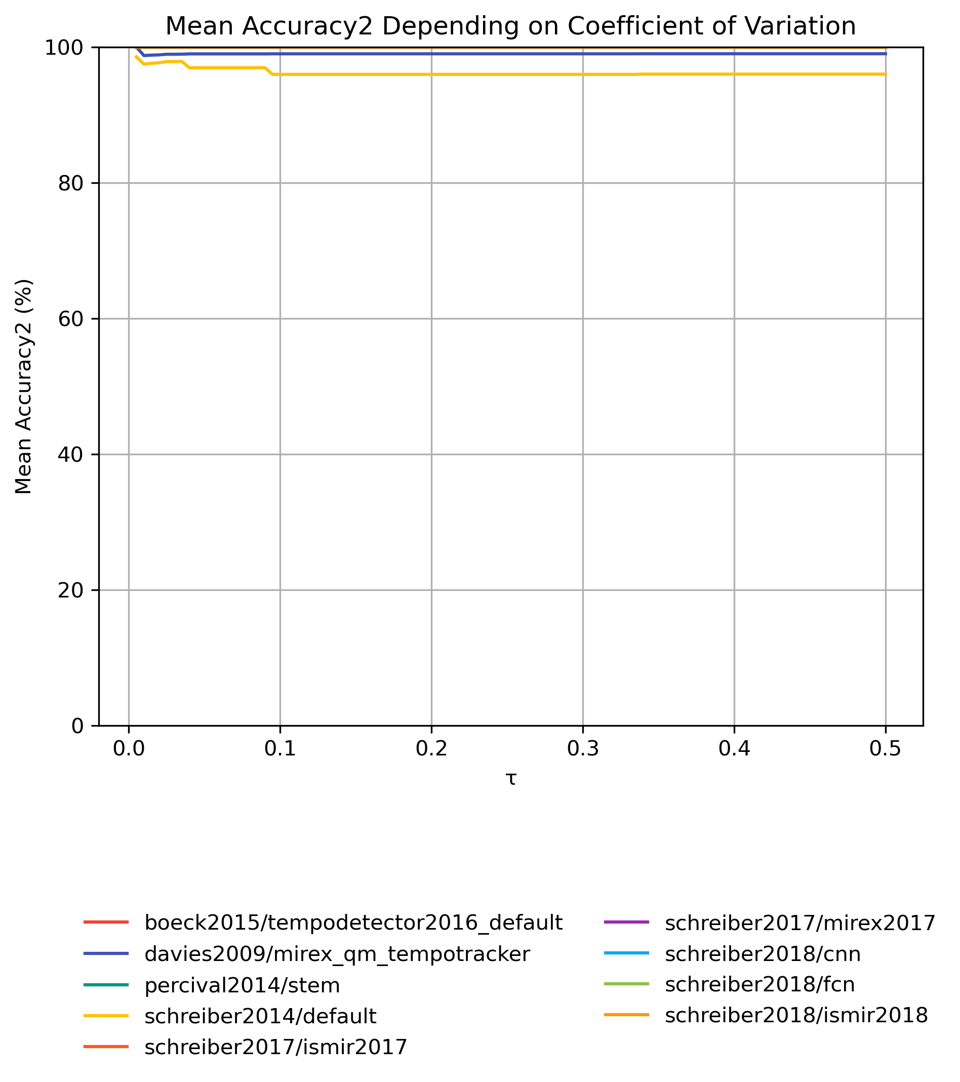
Accuracy2 on cvar-Subsets for 1.0 based on cvar-Values from 1.0
Figure 12: Mean Accuracy2 compared to version 1.0 for tracks with cvar < τ based on beat annotations from 1.0.
CSV JSON LATEX PICKLE SVG PDF PNG
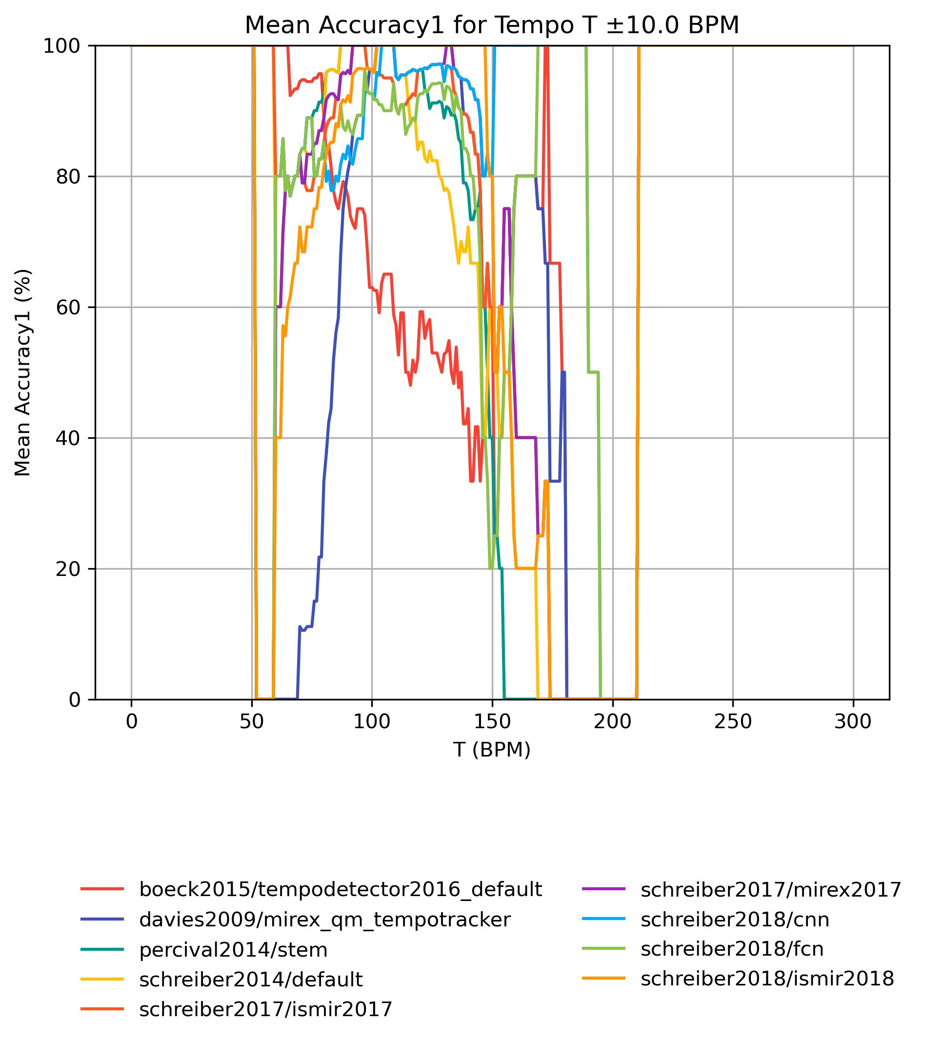
Accuracy1 on Tempo-Subsets
How well does an estimator perform, when only taking a subset of the reference annotations into account? The graphs show mean Accuracy1 for reference subsets with tempi in [T-10,T+10] BPM. Note that the graphs do not show confidence intervals and that some values may be based on very few estimates.
Accuracy1 on Tempo-Subsets for 0.1
Figure 13: Mean Accuracy1 for estimates compared to version 0.1 for tempo intervals around T.
CSV JSON LATEX PICKLE SVG PDF PNG
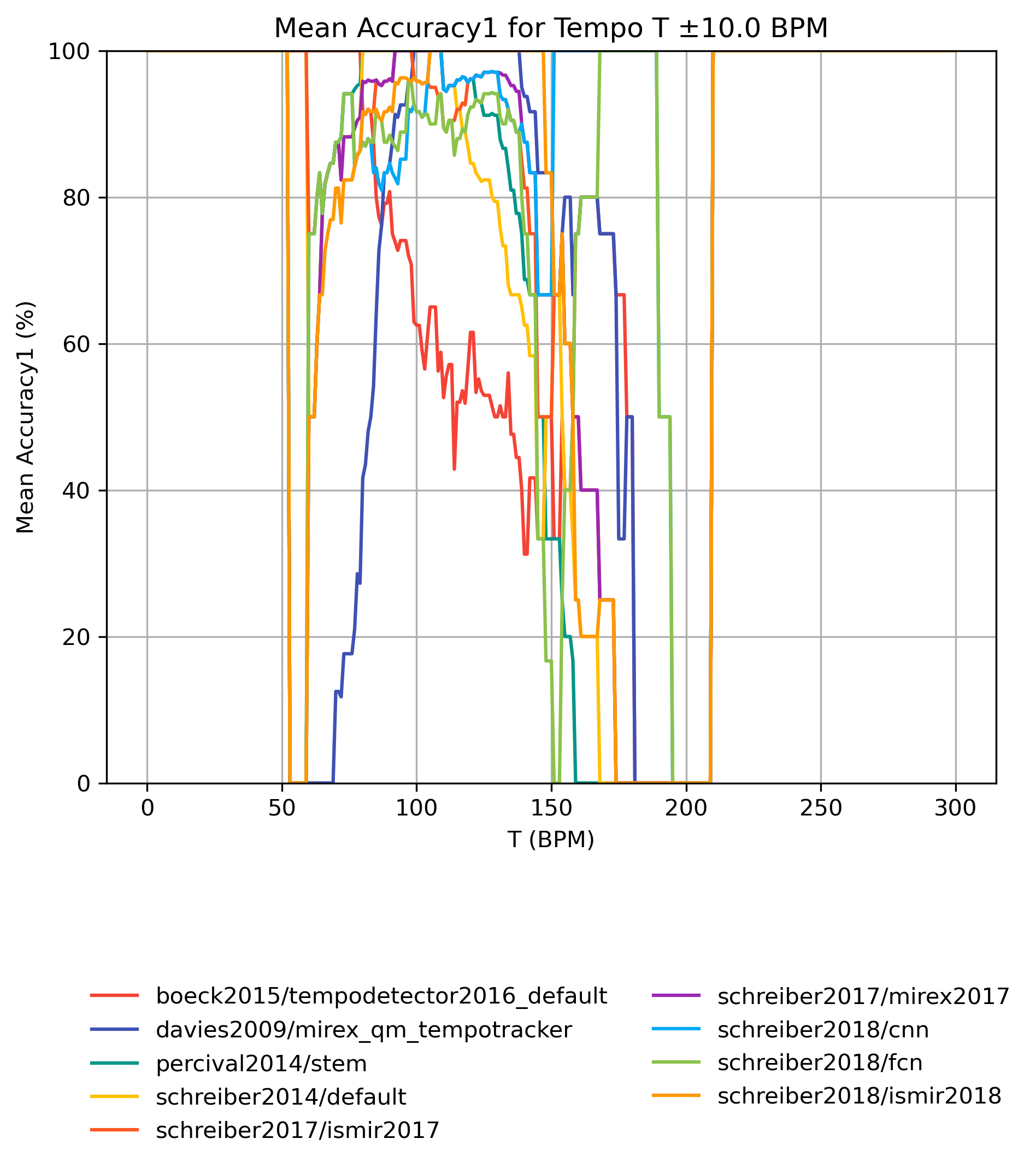
Accuracy1 on Tempo-Subsets for 1.0
Figure 14: Mean Accuracy1 for estimates compared to version 1.0 for tempo intervals around T.
CSV JSON LATEX PICKLE SVG PDF PNG
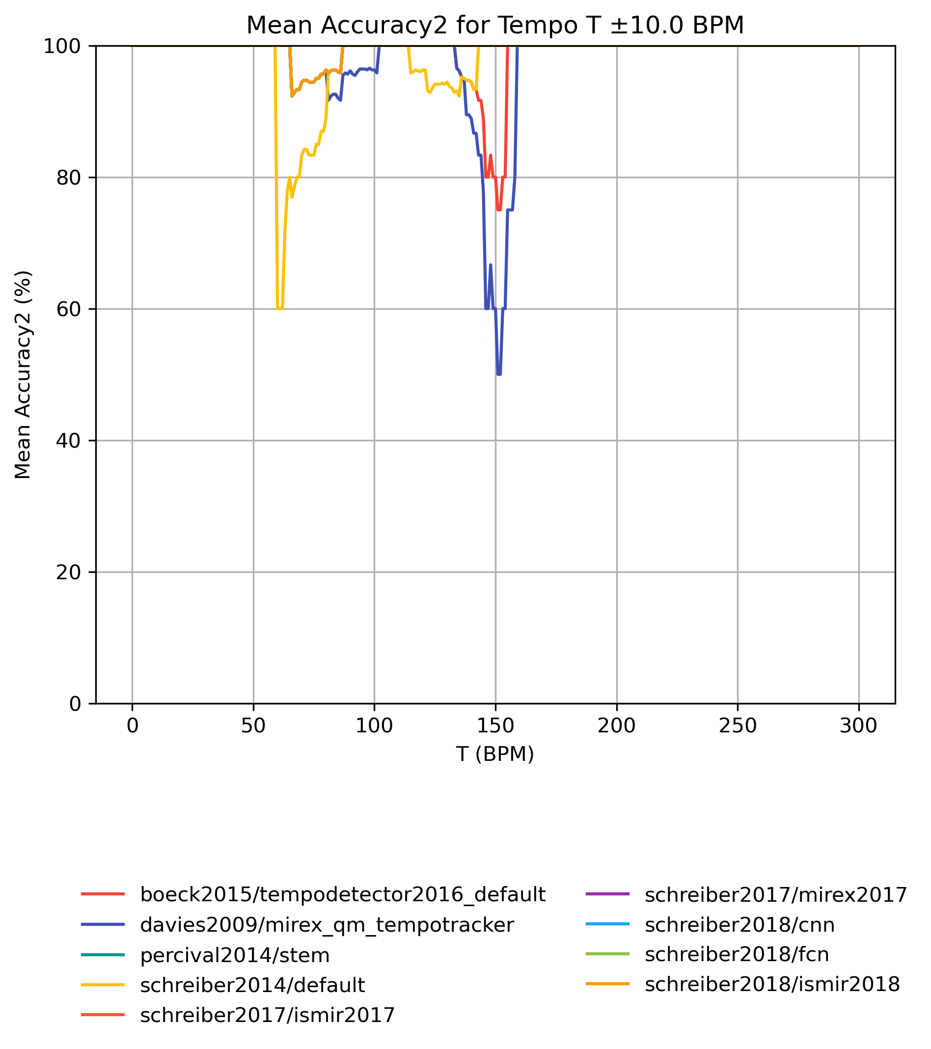
Accuracy2 on Tempo-Subsets
How well does an estimator perform, when only taking a subset of the reference annotations into account? The graphs show mean Accuracy2 for reference subsets with tempi in [T-10,T+10] BPM. Note that the graphs do not show confidence intervals and that some values may be based on very few estimates.
Accuracy2 on Tempo-Subsets for 0.1
Figure 15: Mean Accuracy2 for estimates compared to version 0.1 for tempo intervals around T.
CSV JSON LATEX PICKLE SVG PDF PNG
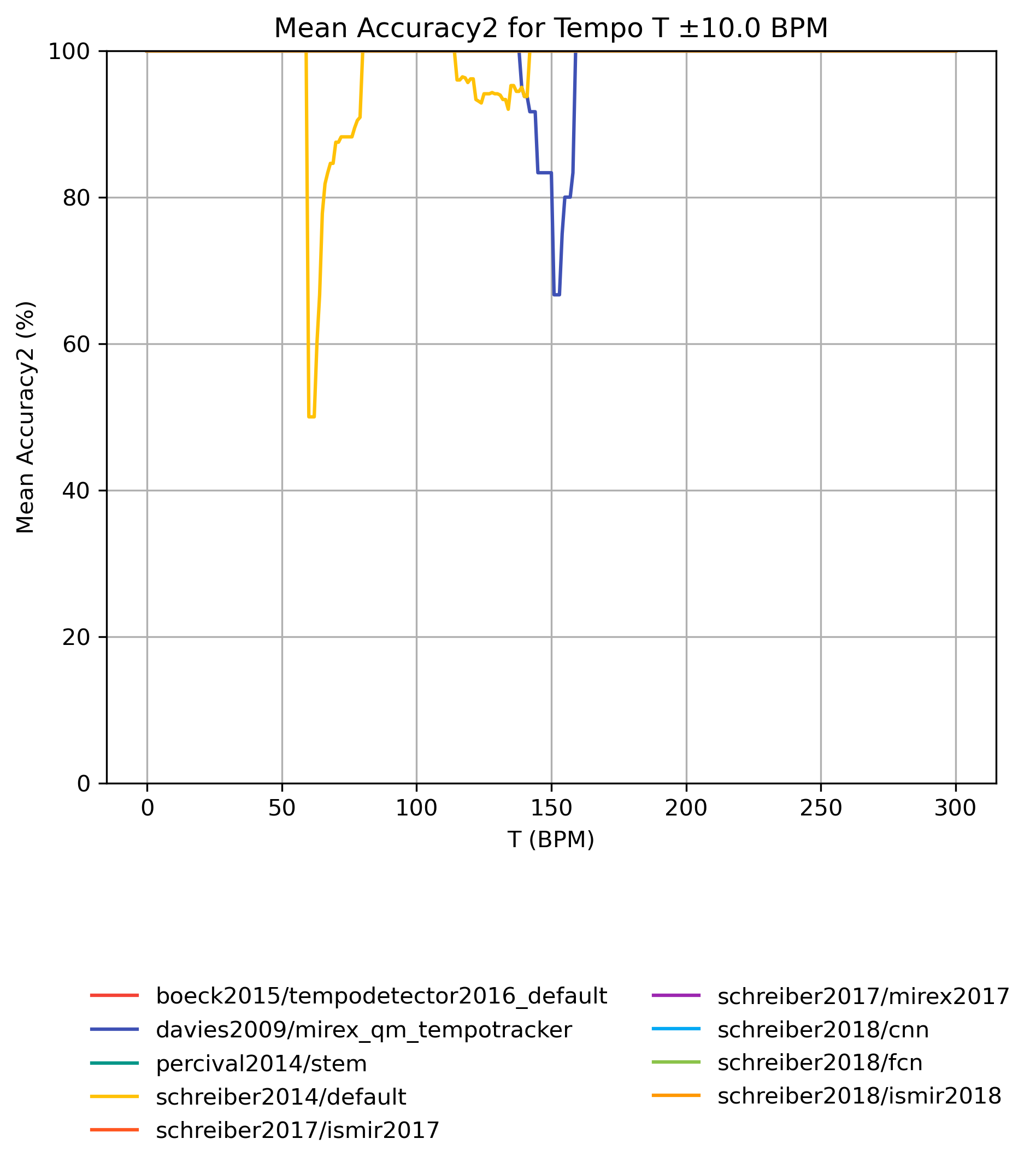
Accuracy2 on Tempo-Subsets for 1.0
Figure 16: Mean Accuracy2 for estimates compared to version 1.0 for tempo intervals around T.
CSV JSON LATEX PICKLE SVG PDF PNG
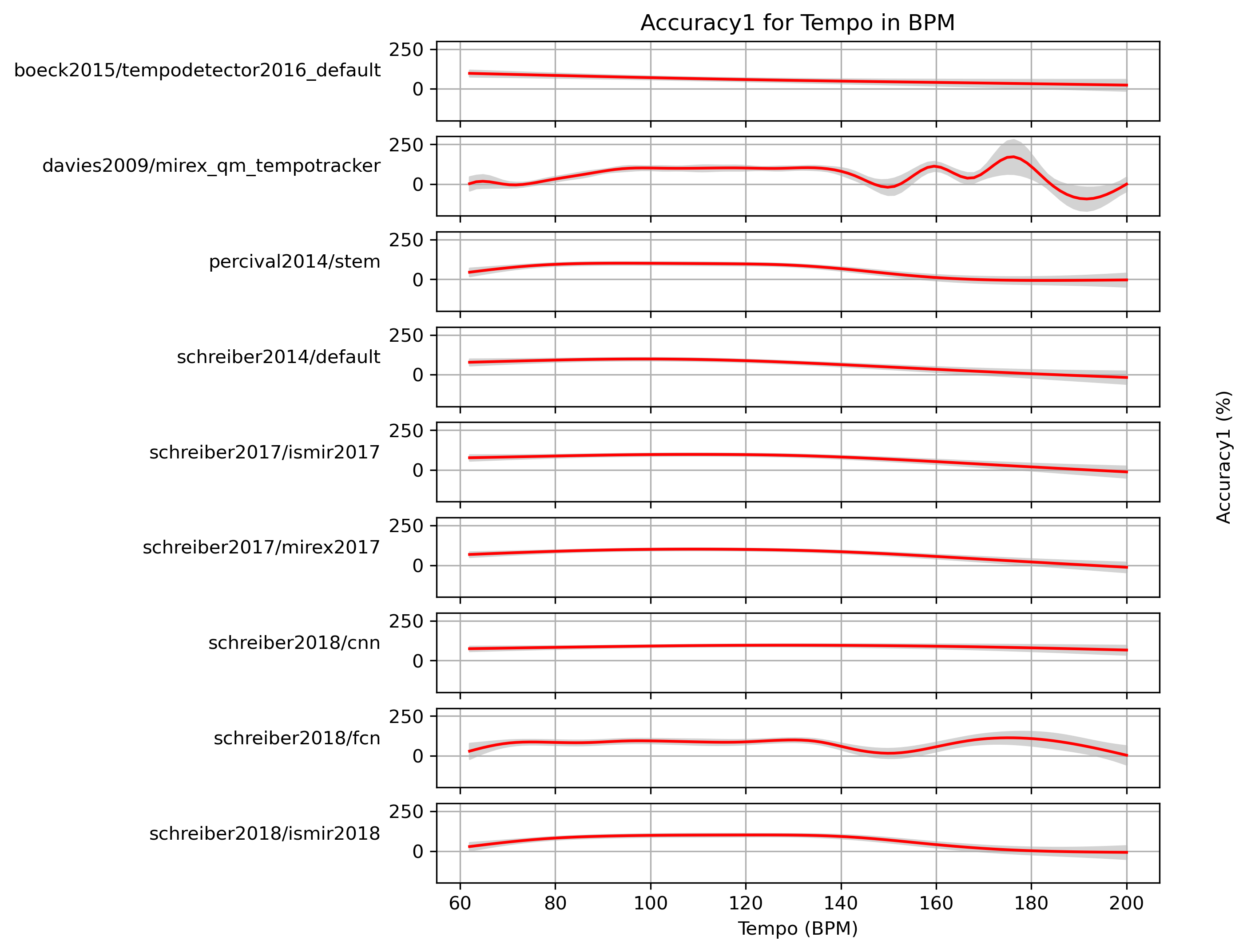
Estimated Accuracy1 for Tempo
When fitting a generalized additive model (GAM) to Accuracy1-values and a ground truth, what Accuracy1 can we expect with confidence?
Estimated Accuracy1 for Tempo for 0.1
Predictions of GAMs trained on Accuracy1 for estimates for reference 0.1.
Figure 17: Accuracy1 predictions of a generalized additive model (GAM) fit to Accuracy1 results for 0.1. The 95% confidence interval around the prediction is shaded in gray.
CSV JSON LATEX PICKLE SVG PDF PNG
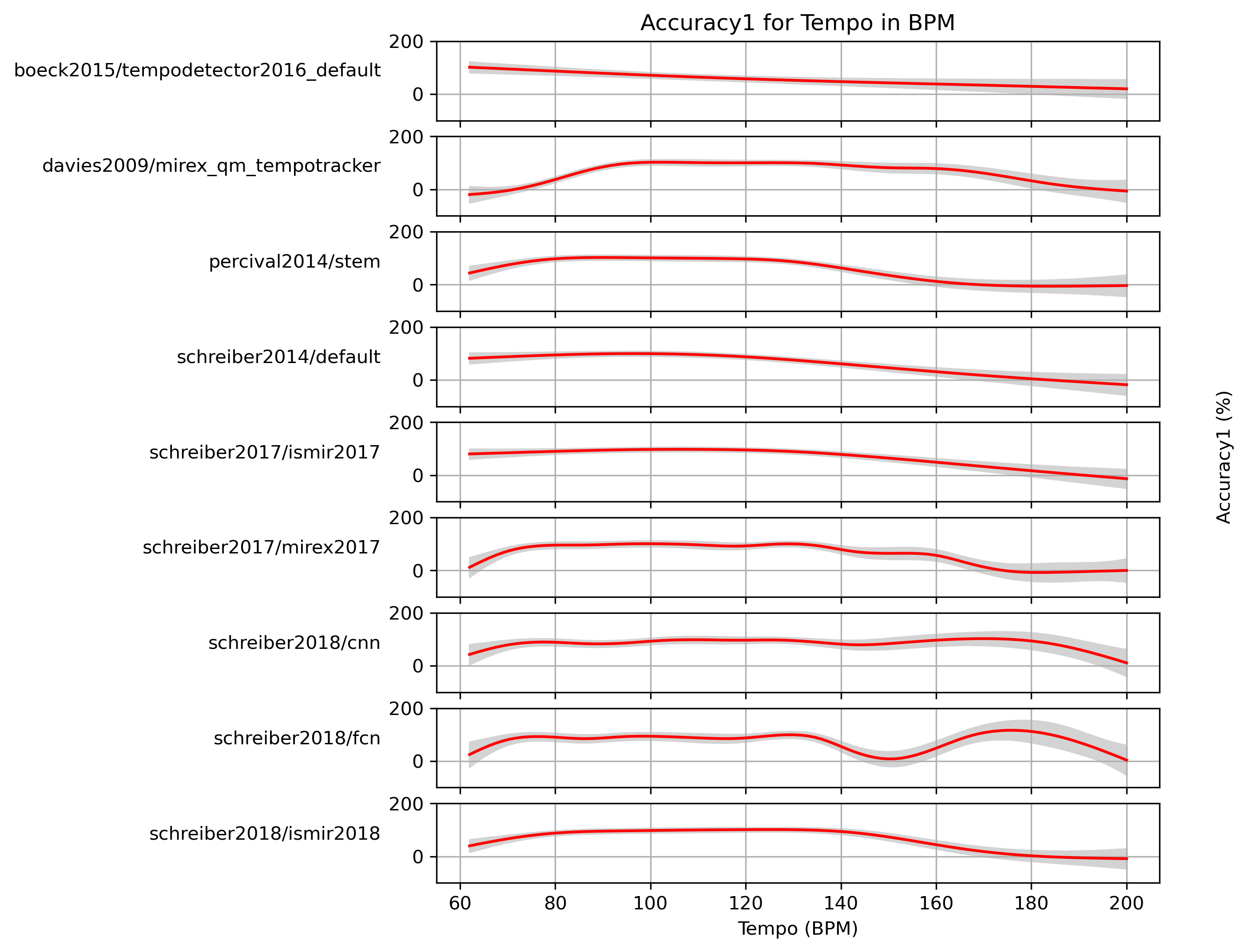
Estimated Accuracy1 for Tempo for 1.0
Predictions of GAMs trained on Accuracy1 for estimates for reference 1.0.
Figure 18: Accuracy1 predictions of a generalized additive model (GAM) fit to Accuracy1 results for 1.0. The 95% confidence interval around the prediction is shaded in gray.
CSV JSON LATEX PICKLE SVG PDF PNG
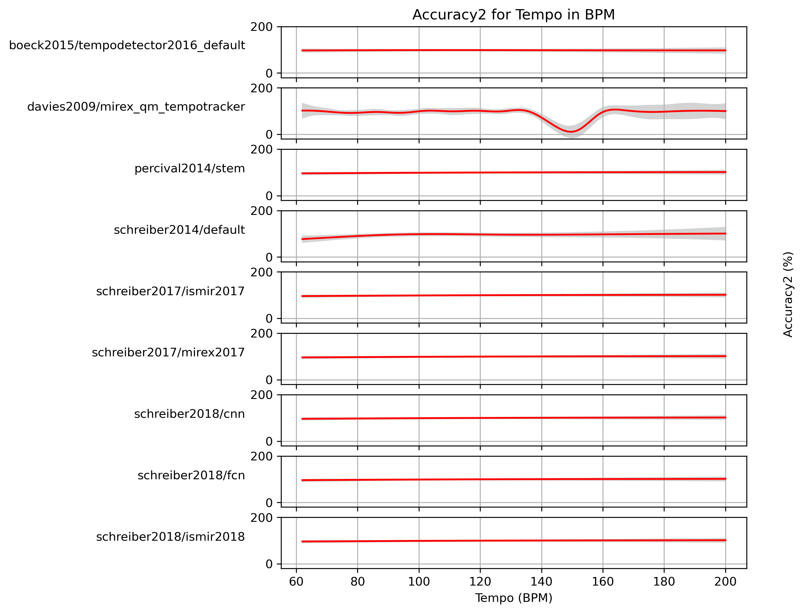
Estimated Accuracy2 for Tempo
When fitting a generalized additive model (GAM) to Accuracy2-values and a ground truth, what Accuracy2 can we expect with confidence?
Estimated Accuracy2 for Tempo for 0.1
Predictions of GAMs trained on Accuracy2 for estimates for reference 0.1.
Figure 19: Accuracy2 predictions of a generalized additive model (GAM) fit to Accuracy2 results for 0.1. The 95% confidence interval around the prediction is shaded in gray.
CSV JSON LATEX PICKLE SVG PDF PNG
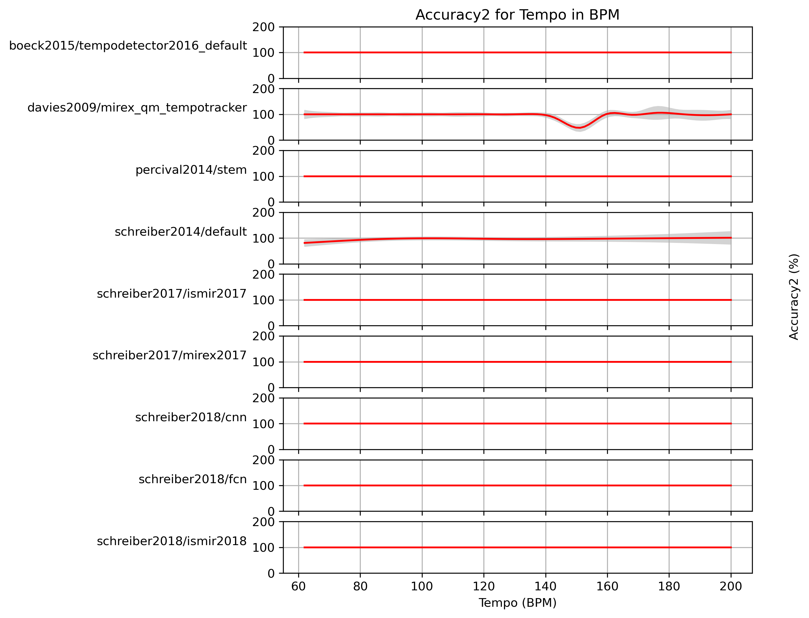
Estimated Accuracy2 for Tempo for 1.0
Predictions of GAMs trained on Accuracy2 for estimates for reference 1.0.
Figure 20: Accuracy2 predictions of a generalized additive model (GAM) fit to Accuracy2 results for 1.0. The 95% confidence interval around the prediction is shaded in gray.
CSV JSON LATEX PICKLE SVG PDF PNG
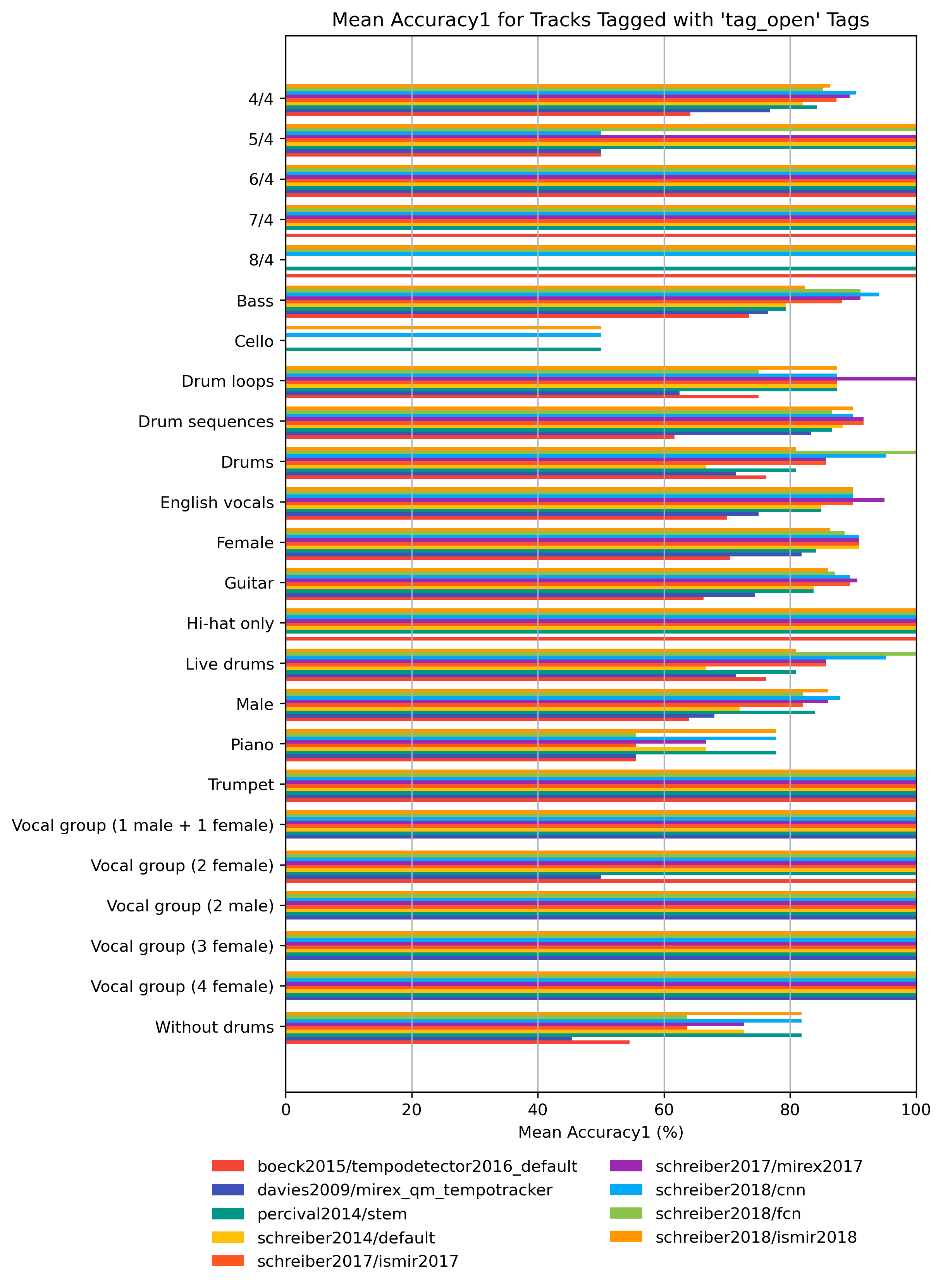
Accuracy1 for ‘tag_open’ Tags
How well does an estimator perform, when only taking tracks into account that are tagged with some kind of label? Note that some values may be based on very few estimates.
Accuracy1 for ‘tag_open’ Tags for 0.1
Figure 21: Mean Accuracy1 of estimates compared to version 0.1 depending on tag from namespace ‘tag_open’.
CSV JSON LATEX PICKLE SVG PDF PNG
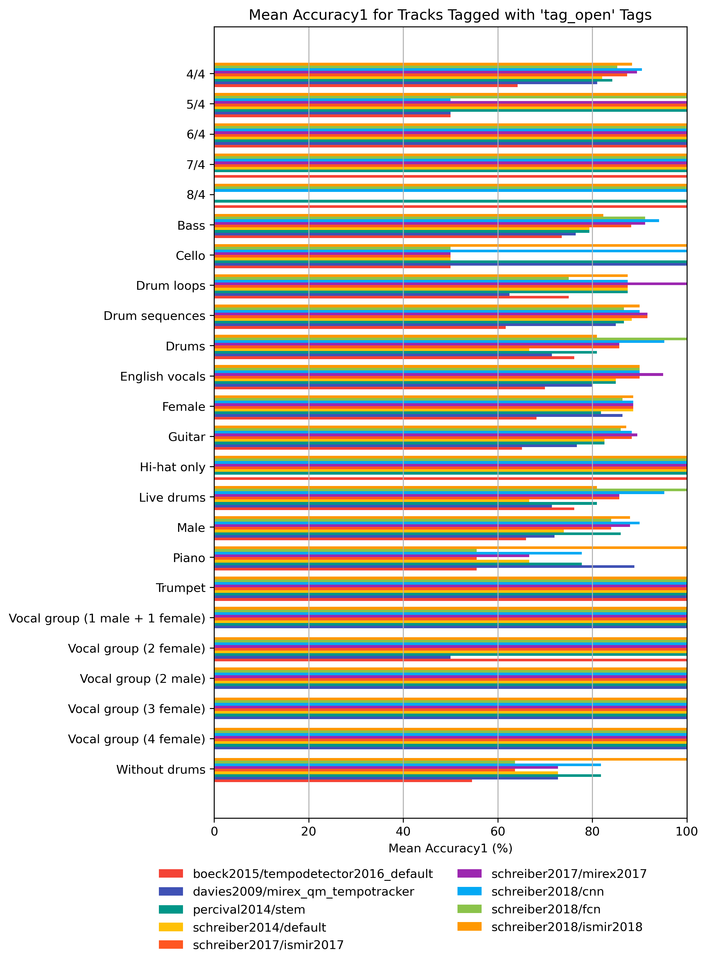
Accuracy1 for ‘tag_open’ Tags for 1.0
Figure 22: Mean Accuracy1 of estimates compared to version 1.0 depending on tag from namespace ‘tag_open’.
CSV JSON LATEX PICKLE SVG PDF PNG
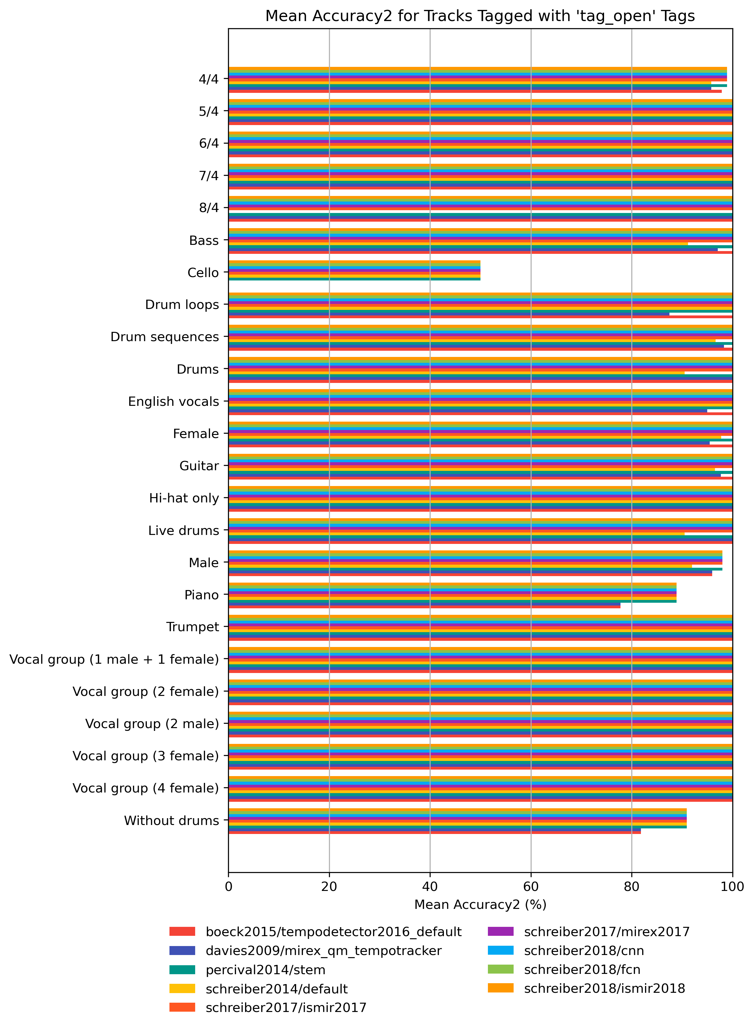
Accuracy2 for ‘tag_open’ Tags
How well does an estimator perform, when only taking tracks into account that are tagged with some kind of label? Note that some values may be based on very few estimates.
Accuracy2 for ‘tag_open’ Tags for 0.1
Figure 23: Mean Accuracy2 of estimates compared to version 0.1 depending on tag from namespace ‘tag_open’.
CSV JSON LATEX PICKLE SVG PDF PNG
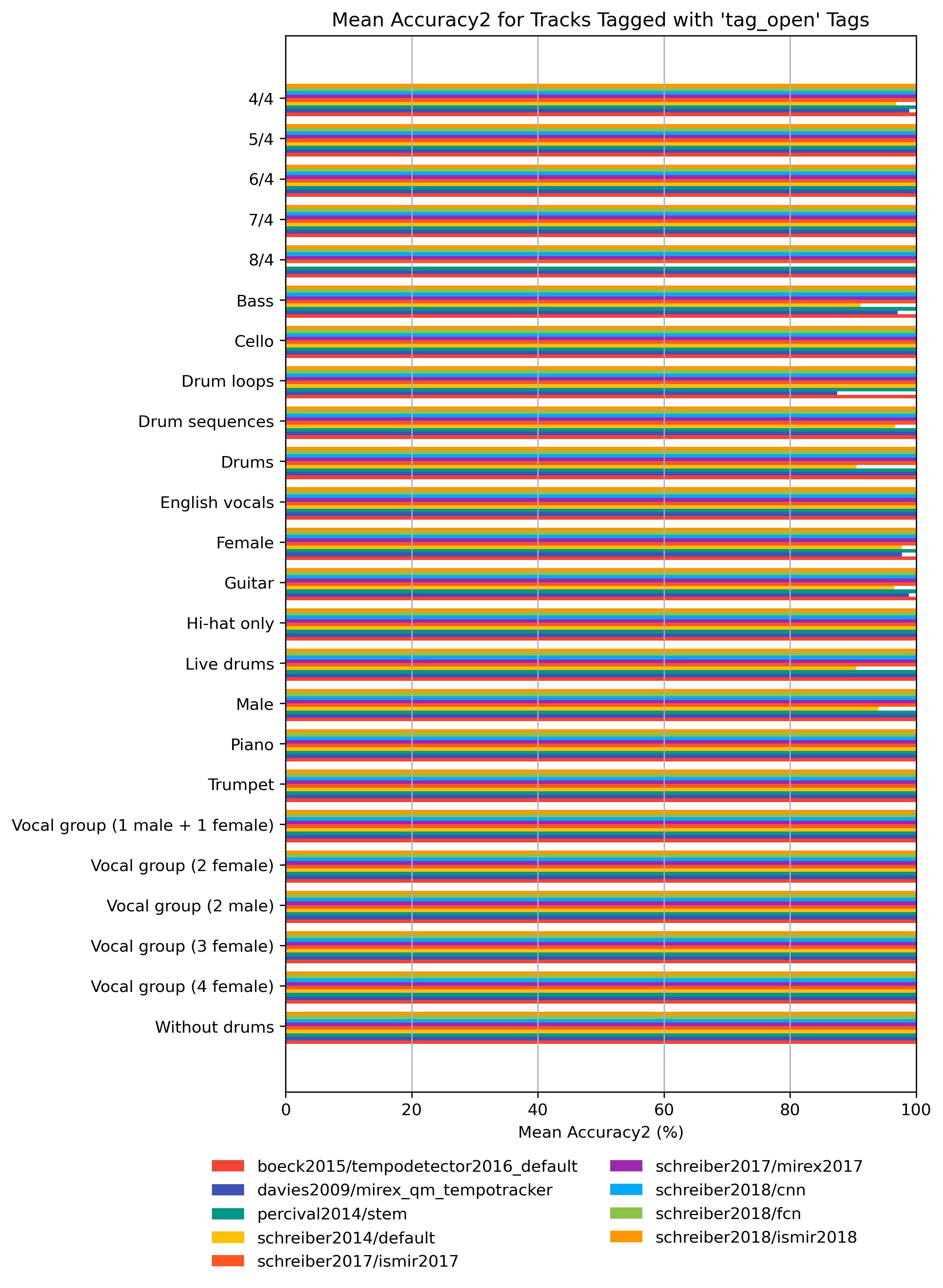
Accuracy2 for ‘tag_open’ Tags for 1.0
Figure 24: Mean Accuracy2 of estimates compared to version 1.0 depending on tag from namespace ‘tag_open’.
CSV JSON LATEX PICKLE SVG PDF PNG
OE1 and OE2
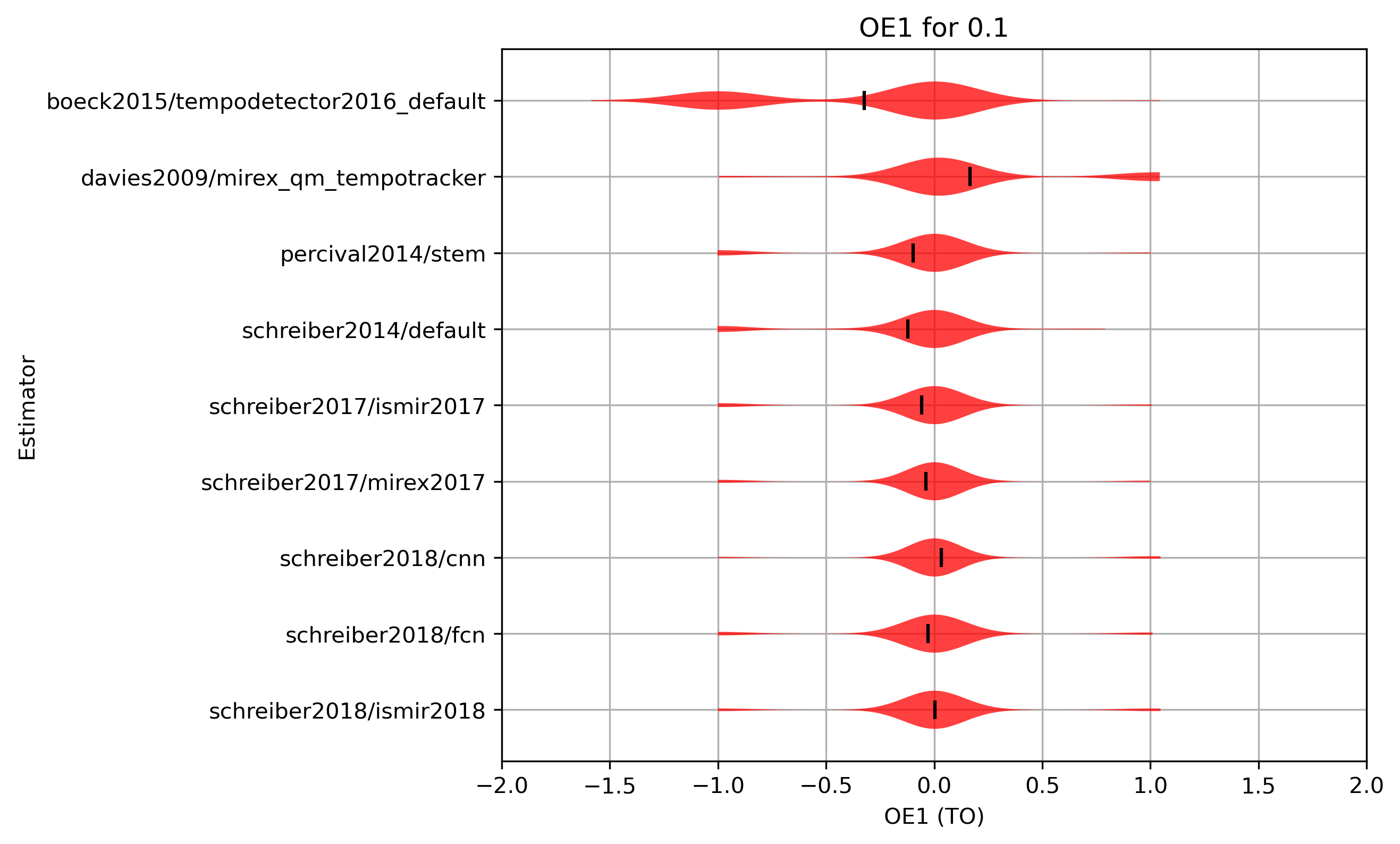
OE1 is defined as octave error between an estimate E and a reference value R.This means that the most common errors—by a factor of 2 or ½—have the same magnitude, namely 1: OE2(E) = log2(E/R).
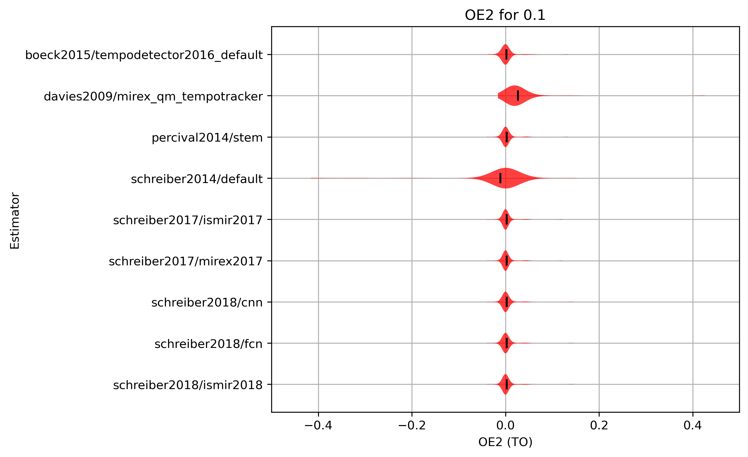
OE2 is the signed OE1 corresponding to the minimum absolute OE1 allowing the octaveerrors 2, 3, 1/2, and 1/3: OE2(E) = arg minx(|x|) with x ∈ {OE1(E), OE1(2E), OE1(3E), OE1(½E), OE1(⅓E)}
Mean OE1/OE2 Results for 0.1
| Estimator | OE1_MEAN | OE1_STDEV | OE2_MEAN | OE2_STDEV |
|---|---|---|---|---|
| schreiber2018/cnn | 0.0328 | 0.3003 | 0.0028 | 0.0170 |
| schreiber2017/mirex2017 | -0.0375 | 0.3121 | 0.0025 | 0.0153 |
| schreiber2017/ismir2017 | -0.0575 | 0.3401 | 0.0025 | 0.0153 |
| schreiber2018/ismir2018 | 0.0026 | 0.3477 | 0.0026 | 0.0170 |
| schreiber2014/default | -0.1211 | 0.3563 | -0.0111 | 0.0715 |
| schreiber2018/fcn | -0.0274 | 0.3593 | 0.0026 | 0.0171 |
| percival2014/stem | -0.0973 | 0.3610 | 0.0027 | 0.0164 |
| davies2009/mirex_qm_tempotracker | 0.1665 | 0.4421 | 0.0265 | 0.0442 |
| boeck2015/tempodetector2016_default | -0.3235 | 0.5013 | 0.0024 | 0.0171 |
Table 9: Mean OE1/OE2 for estimates compared to version 0.1 ordered by standard deviation.
Raw data OE1: CSV JSON LATEX PICKLE
Raw data OE2: CSV JSON LATEX PICKLE
OE1 distribution for 0.1
Figure 25: OE1 for estimates compared to version 0.1. Shown are the mean OE1 and an empirical distribution of the sample, using kernel density estimation (KDE).
CSV JSON LATEX PICKLE SVG PDF PNG
OE2 distribution for 0.1
Figure 26: OE2 for estimates compared to version 0.1. Shown are the mean OE2 and an empirical distribution of the sample, using kernel density estimation (KDE).
CSV JSON LATEX PICKLE SVG PDF PNG
Mean OE1/OE2 Results for 1.0
| Estimator | OE1_MEAN | OE1_STDEV | OE2_MEAN | OE2_STDEV |
|---|---|---|---|---|
| schreiber2018/cnn | 0.0203 | 0.3155 | 0.0003 | 0.0031 |
| schreiber2017/mirex2017 | -0.0499 | 0.3281 | 0.0001 | 0.0019 |
| schreiber2018/ismir2018 | -0.0098 | 0.3318 | 0.0002 | 0.0029 |
| schreiber2017/ismir2017 | -0.0699 | 0.3541 | 0.0001 | 0.0019 |
| schreiber2014/default | -0.1335 | 0.3677 | -0.0135 | 0.0687 |
| percival2014/stem | -0.1098 | 0.3720 | 0.0002 | 0.0027 |
| schreiber2018/fcn | -0.0398 | 0.3725 | 0.0002 | 0.0035 |
| davies2009/mirex_qm_tempotracker | 0.1541 | 0.4339 | 0.0241 | 0.0415 |
| boeck2015/tempodetector2016_default | -0.3359 | 0.5021 | -0.0001 | 0.0054 |
Table 10: Mean OE1/OE2 for estimates compared to version 1.0 ordered by standard deviation.
Raw data OE1: CSV JSON LATEX PICKLE
Raw data OE2: CSV JSON LATEX PICKLE
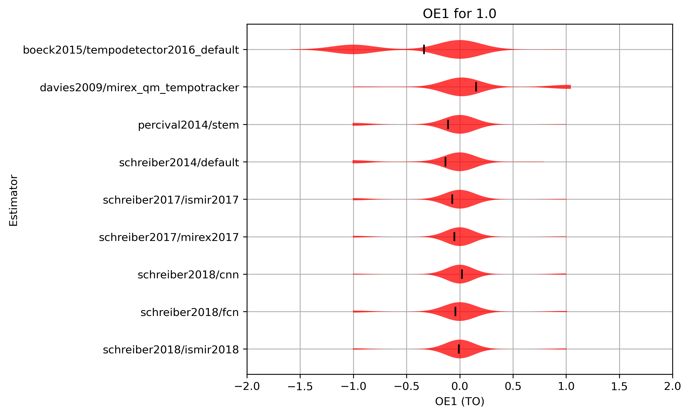
OE1 distribution for 1.0
Figure 27: OE1 for estimates compared to version 1.0. Shown are the mean OE1 and an empirical distribution of the sample, using kernel density estimation (KDE).
CSV JSON LATEX PICKLE SVG PDF PNG
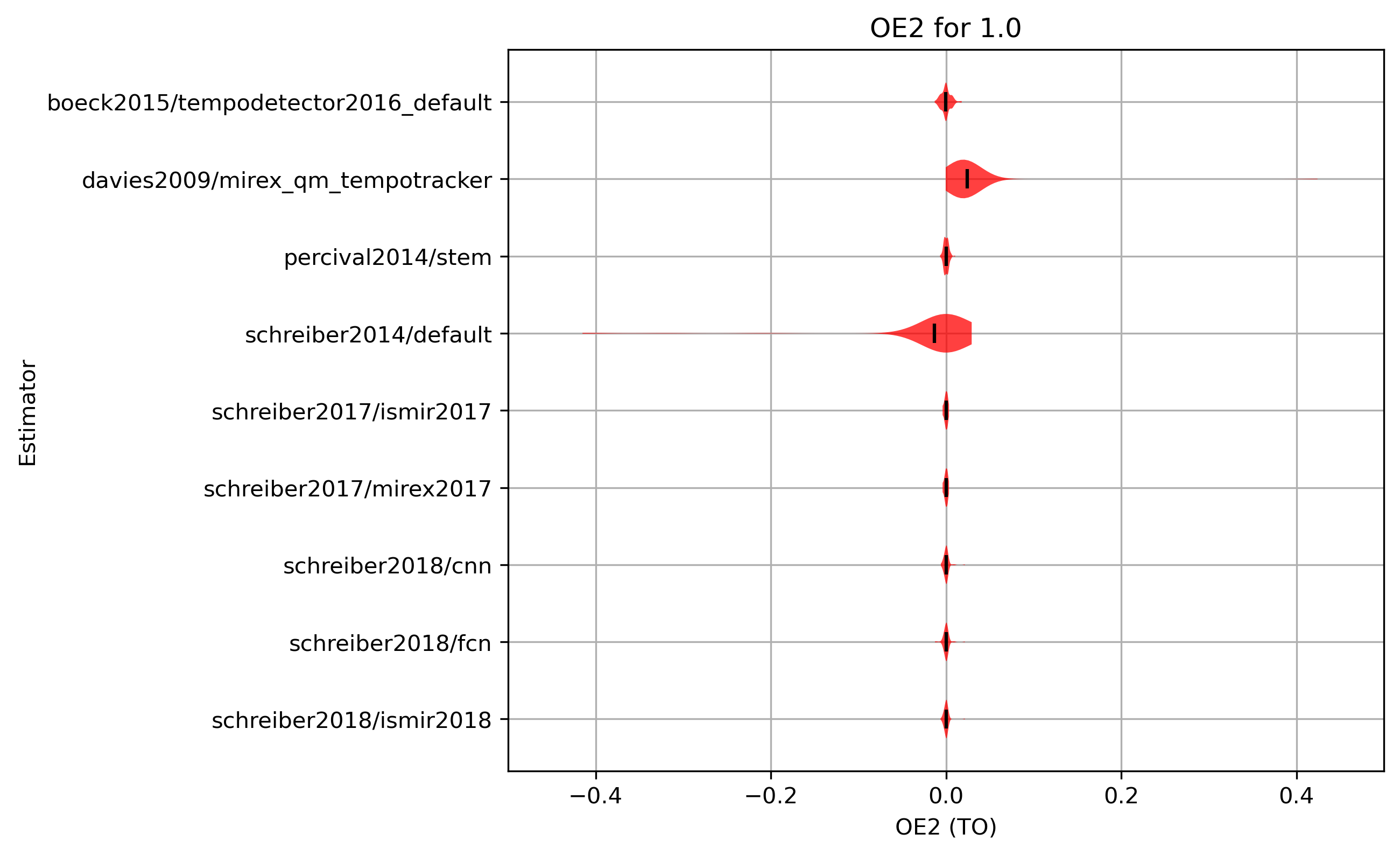
OE2 distribution for 1.0
Figure 28: OE2 for estimates compared to version 1.0. Shown are the mean OE2 and an empirical distribution of the sample, using kernel density estimation (KDE).
CSV JSON LATEX PICKLE SVG PDF PNG
Significance of Differences
| Estimator | boeck2015/tempodetector2016_default | davies2009/mirex_qm_tempotracker | percival2014/stem | schreiber2014/default | schreiber2017/ismir2017 | schreiber2017/mirex2017 | schreiber2018/cnn | schreiber2018/fcn | schreiber2018/ismir2018 |
|---|---|---|---|---|---|---|---|---|---|
| boeck2015/tempodetector2016_default | 1.0000 | 0.0000 | 0.0001 | 0.0001 | 0.0000 | 0.0000 | 0.0000 | 0.0000 | 0.0000 |
| davies2009/mirex_qm_tempotracker | 0.0000 | 1.0000 | 0.0000 | 0.0000 | 0.0000 | 0.0000 | 0.0049 | 0.0001 | 0.0001 |
| percival2014/stem | 0.0001 | 0.0000 | 1.0000 | 0.4618 | 0.2522 | 0.0580 | 0.0006 | 0.0710 | 0.0013 |
| schreiber2014/default | 0.0001 | 0.0000 | 0.4618 | 1.0000 | 0.0300 | 0.0040 | 0.0001 | 0.0319 | 0.0012 |
| schreiber2017/ismir2017 | 0.0000 | 0.0000 | 0.2522 | 0.0300 | 1.0000 | 0.3197 | 0.0116 | 0.4061 | 0.0569 |
| schreiber2017/mirex2017 | 0.0000 | 0.0000 | 0.0580 | 0.0040 | 0.3197 | 1.0000 | 0.0507 | 0.7957 | 0.1574 |
| schreiber2018/cnn | 0.0000 | 0.0049 | 0.0006 | 0.0001 | 0.0116 | 0.0507 | 1.0000 | 0.0330 | 0.4058 |
| schreiber2018/fcn | 0.0000 | 0.0001 | 0.0710 | 0.0319 | 0.4061 | 0.7957 | 0.0330 | 1.0000 | 0.4696 |
| schreiber2018/ismir2018 | 0.0000 | 0.0001 | 0.0013 | 0.0012 | 0.0569 | 0.1574 | 0.4058 | 0.4696 | 1.0000 |
Table 11: Paired t-test p-values, using reference annotations 1.0 as groundtruth with OE1. H0: the true mean difference between paired samples is zero. If p<=ɑ, reject H0, i.e. we have a significant difference between estimates from the two algorithms. In the table, p-values<0.05 are set in bold.
| Estimator | boeck2015/tempodetector2016_default | davies2009/mirex_qm_tempotracker | percival2014/stem | schreiber2014/default | schreiber2017/ismir2017 | schreiber2017/mirex2017 | schreiber2018/cnn | schreiber2018/fcn | schreiber2018/ismir2018 |
|---|---|---|---|---|---|---|---|---|---|
| boeck2015/tempodetector2016_default | 1.0000 | 0.0000 | 0.0001 | 0.0001 | 0.0000 | 0.0000 | 0.0000 | 0.0000 | 0.0000 |
| davies2009/mirex_qm_tempotracker | 0.0000 | 1.0000 | 0.0000 | 0.0000 | 0.0000 | 0.0000 | 0.0049 | 0.0001 | 0.0001 |
| percival2014/stem | 0.0001 | 0.0000 | 1.0000 | 0.4618 | 0.2522 | 0.0580 | 0.0006 | 0.0710 | 0.0013 |
| schreiber2014/default | 0.0001 | 0.0000 | 0.4618 | 1.0000 | 0.0300 | 0.0040 | 0.0001 | 0.0319 | 0.0012 |
| schreiber2017/ismir2017 | 0.0000 | 0.0000 | 0.2522 | 0.0300 | 1.0000 | 0.3197 | 0.0116 | 0.4061 | 0.0569 |
| schreiber2017/mirex2017 | 0.0000 | 0.0000 | 0.0580 | 0.0040 | 0.3197 | 1.0000 | 0.0507 | 0.7957 | 0.1574 |
| schreiber2018/cnn | 0.0000 | 0.0049 | 0.0006 | 0.0001 | 0.0116 | 0.0507 | 1.0000 | 0.0330 | 0.4058 |
| schreiber2018/fcn | 0.0000 | 0.0001 | 0.0710 | 0.0319 | 0.4061 | 0.7957 | 0.0330 | 1.0000 | 0.4696 |
| schreiber2018/ismir2018 | 0.0000 | 0.0001 | 0.0013 | 0.0012 | 0.0569 | 0.1574 | 0.4058 | 0.4696 | 1.0000 |
Table 12: Paired t-test p-values, using reference annotations 0.1 as groundtruth with OE1. H0: the true mean difference between paired samples is zero. If p<=ɑ, reject H0, i.e. we have a significant difference between estimates from the two algorithms. In the table, p-values<0.05 are set in bold.
| Estimator | boeck2015/tempodetector2016_default | davies2009/mirex_qm_tempotracker | percival2014/stem | schreiber2014/default | schreiber2017/ismir2017 | schreiber2017/mirex2017 | schreiber2018/cnn | schreiber2018/fcn | schreiber2018/ismir2018 |
|---|---|---|---|---|---|---|---|---|---|
| boeck2015/tempodetector2016_default | 1.0000 | 0.0000 | 0.5752 | 0.0536 | 0.7522 | 0.7522 | 0.4778 | 0.6639 | 0.6508 |
| davies2009/mirex_qm_tempotracker | 0.0000 | 1.0000 | 0.0000 | 0.0000 | 0.0000 | 0.0000 | 0.0000 | 0.0000 | 0.0000 |
| percival2014/stem | 0.5752 | 0.0000 | 1.0000 | 0.0509 | 0.5002 | 0.5002 | 0.7342 | 0.8953 | 0.8052 |
| schreiber2014/default | 0.0536 | 0.0000 | 0.0509 | 1.0000 | 0.0524 | 0.0524 | 0.0481 | 0.0504 | 0.0506 |
| schreiber2017/ismir2017 | 0.7522 | 0.0000 | 0.5002 | 0.0524 | 1.0000 | 0.4277 | 0.4172 | 0.7474 | 0.7364 |
| schreiber2017/mirex2017 | 0.7522 | 0.0000 | 0.5002 | 0.0524 | 0.4277 | 1.0000 | 0.4172 | 0.7474 | 0.7364 |
| schreiber2018/cnn | 0.4778 | 0.0000 | 0.7342 | 0.0481 | 0.4172 | 0.4172 | 1.0000 | 0.5465 | 0.4596 |
| schreiber2018/fcn | 0.6639 | 0.0000 | 0.8953 | 0.0504 | 0.7474 | 0.7474 | 0.5465 | 1.0000 | 0.9230 |
| schreiber2018/ismir2018 | 0.6508 | 0.0000 | 0.8052 | 0.0506 | 0.7364 | 0.7364 | 0.4596 | 0.9230 | 1.0000 |
Table 13: Paired t-test p-values, using reference annotations 1.0 as groundtruth with OE2. H0: the true mean difference between paired samples is zero. If p<=ɑ, reject H0, i.e. we have a significant difference between estimates from the two algorithms. In the table, p-values<0.05 are set in bold.
| Estimator | boeck2015/tempodetector2016_default | davies2009/mirex_qm_tempotracker | percival2014/stem | schreiber2014/default | schreiber2017/ismir2017 | schreiber2017/mirex2017 | schreiber2018/cnn | schreiber2018/fcn | schreiber2018/ismir2018 |
|---|---|---|---|---|---|---|---|---|---|
| boeck2015/tempodetector2016_default | 1.0000 | 0.0000 | 0.5752 | 0.0536 | 0.7522 | 0.7522 | 0.4778 | 0.6639 | 0.6508 |
| davies2009/mirex_qm_tempotracker | 0.0000 | 1.0000 | 0.0000 | 0.0000 | 0.0000 | 0.0000 | 0.0000 | 0.0000 | 0.0000 |
| percival2014/stem | 0.5752 | 0.0000 | 1.0000 | 0.0509 | 0.5002 | 0.5002 | 0.7342 | 0.8953 | 0.8052 |
| schreiber2014/default | 0.0536 | 0.0000 | 0.0509 | 1.0000 | 0.0524 | 0.0524 | 0.0481 | 0.0504 | 0.0506 |
| schreiber2017/ismir2017 | 0.7522 | 0.0000 | 0.5002 | 0.0524 | 1.0000 | 0.4277 | 0.4172 | 0.7474 | 0.7364 |
| schreiber2017/mirex2017 | 0.7522 | 0.0000 | 0.5002 | 0.0524 | 0.4277 | 1.0000 | 0.4172 | 0.7474 | 0.7364 |
| schreiber2018/cnn | 0.4778 | 0.0000 | 0.7342 | 0.0481 | 0.4172 | 0.4172 | 1.0000 | 0.5465 | 0.4596 |
| schreiber2018/fcn | 0.6639 | 0.0000 | 0.8953 | 0.0504 | 0.7474 | 0.7474 | 0.5465 | 1.0000 | 0.9230 |
| schreiber2018/ismir2018 | 0.6508 | 0.0000 | 0.8052 | 0.0506 | 0.7364 | 0.7364 | 0.4596 | 0.9230 | 1.0000 |
Table 14: Paired t-test p-values, using reference annotations 0.1 as groundtruth with OE2. H0: the true mean difference between paired samples is zero. If p<=ɑ, reject H0, i.e. we have a significant difference between estimates from the two algorithms. In the table, p-values<0.05 are set in bold.
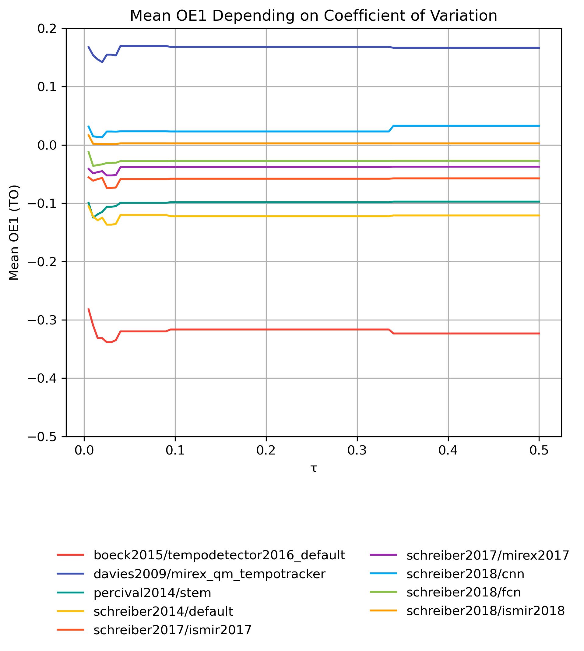
OE1 on cvar-Subsets
How well does an estimator perform, when only taking tracks into account that have a cvar-value of less than τ, i.e., have a more or less stable beat?
OE1 on cvar-Subsets for 0.1 based on cvar-Values from 1.0
Figure 29: Mean OE1 compared to version 0.1 for tracks with cvar < τ based on beat annotations from 0.1.
CSV JSON LATEX PICKLE SVG PDF PNG
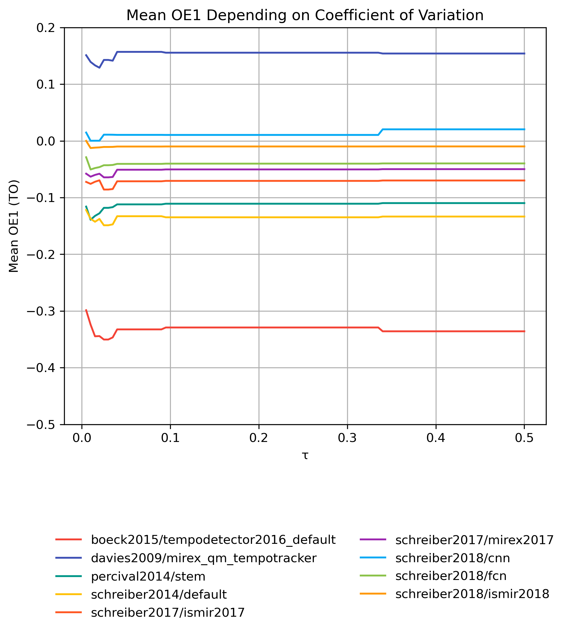
OE1 on cvar-Subsets for 1.0 based on cvar-Values from 1.0
Figure 30: Mean OE1 compared to version 1.0 for tracks with cvar < τ based on beat annotations from 1.0.
CSV JSON LATEX PICKLE SVG PDF PNG
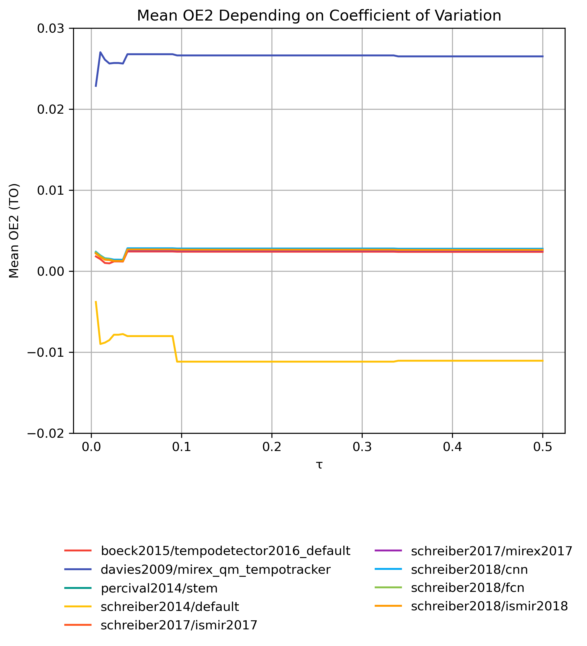
OE2 on cvar-Subsets
How well does an estimator perform, when only taking tracks into account that have a cvar-value of less than τ, i.e., have a more or less stable beat?
OE2 on cvar-Subsets for 0.1 based on cvar-Values from 1.0
Figure 31: Mean OE2 compared to version 0.1 for tracks with cvar < τ based on beat annotations from 0.1.
CSV JSON LATEX PICKLE SVG PDF PNG
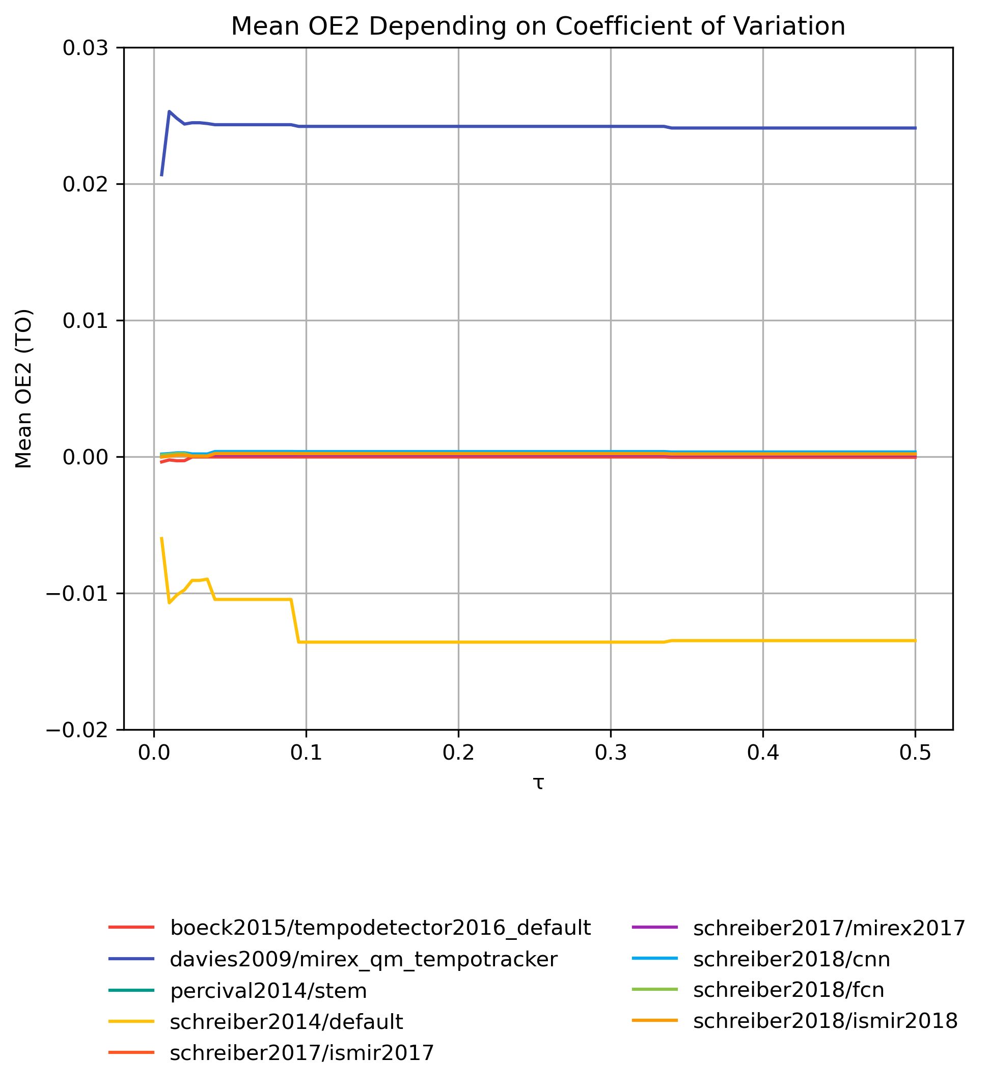
OE2 on cvar-Subsets for 1.0 based on cvar-Values from 1.0
Figure 32: Mean OE2 compared to version 1.0 for tracks with cvar < τ based on beat annotations from 1.0.
CSV JSON LATEX PICKLE SVG PDF PNG
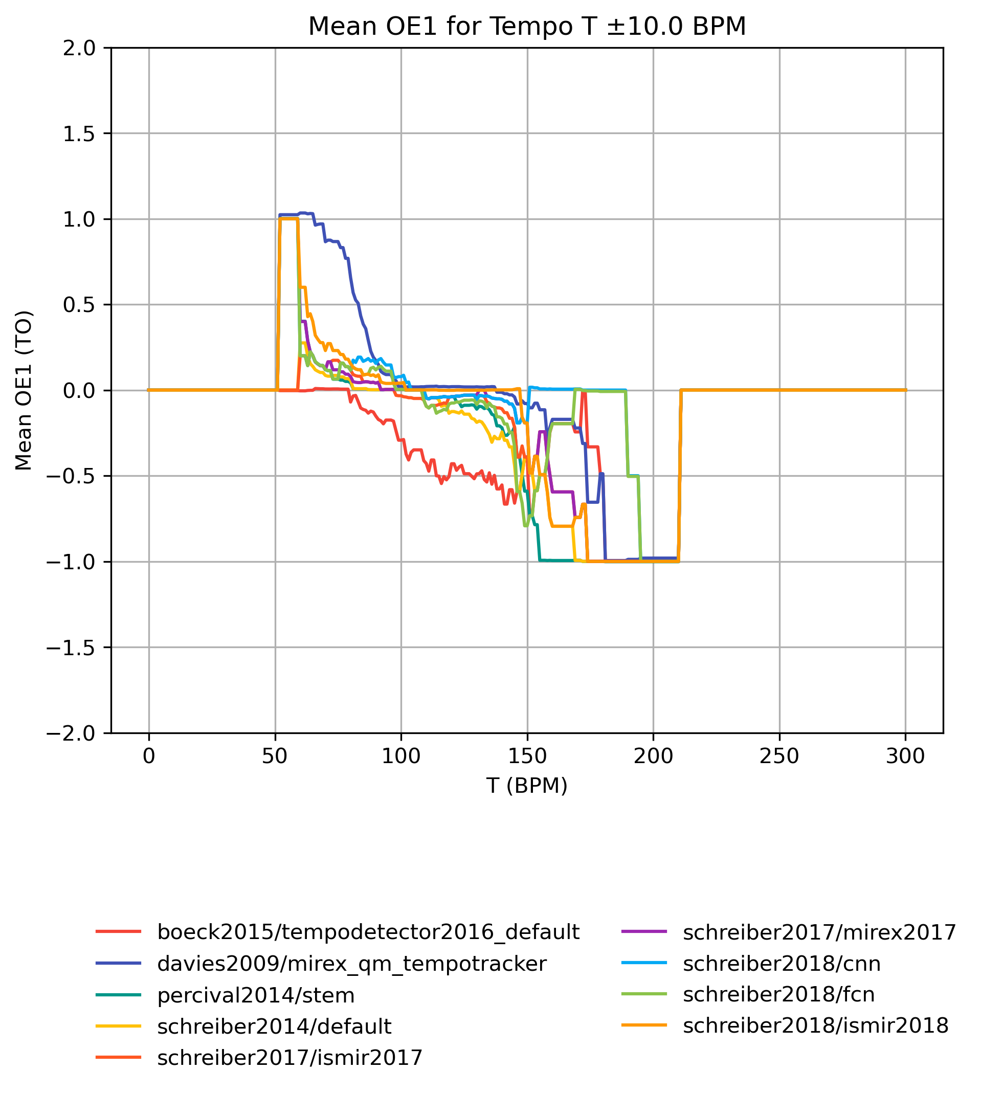
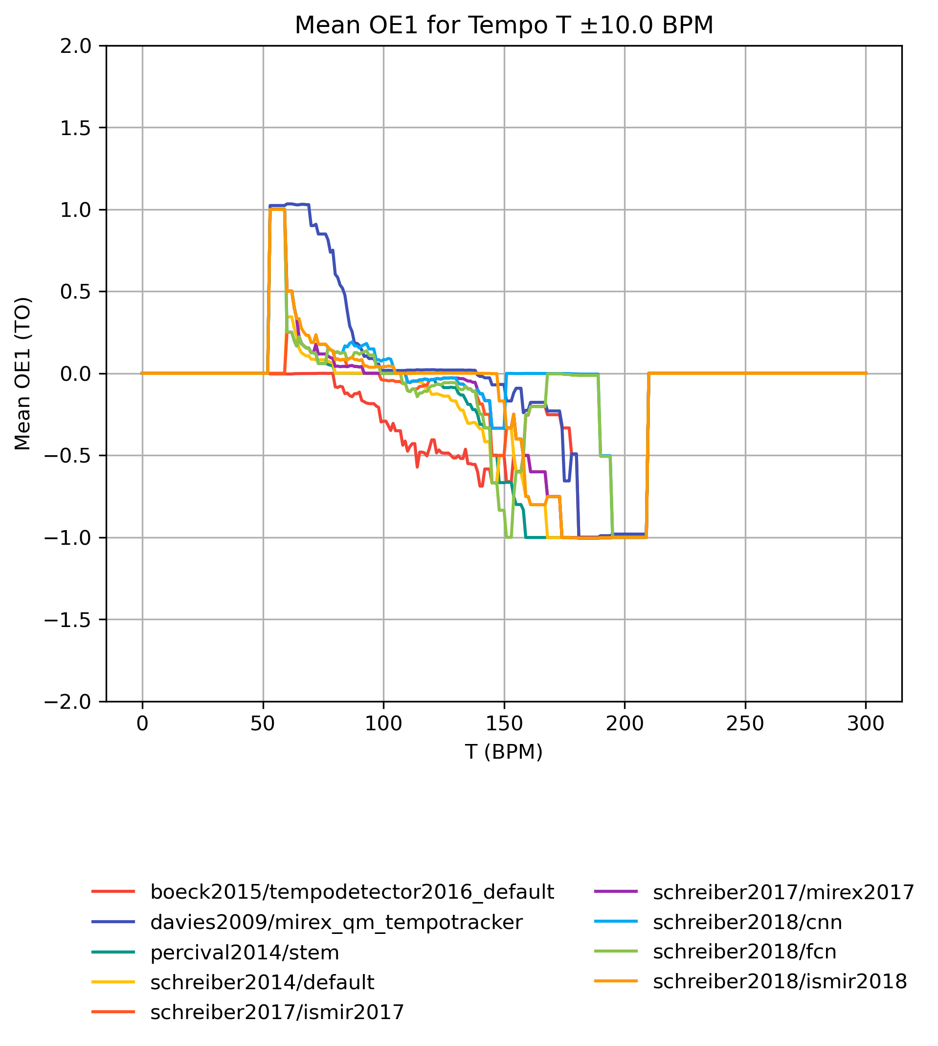
OE1 on Tempo-Subsets
How well does an estimator perform, when only taking a subset of the reference annotations into account? The graphs show mean OE1 for reference subsets with tempi in [T-10,T+10] BPM. Note that the graphs do not show confidence intervals and that some values may be based on very few estimates.
OE1 on Tempo-Subsets for 0.1
Figure 33: Mean OE1 for estimates compared to version 0.1 for tempo intervals around T.
CSV JSON LATEX PICKLE SVG PDF PNG
OE1 on Tempo-Subsets for 1.0
Figure 34: Mean OE1 for estimates compared to version 1.0 for tempo intervals around T.
CSV JSON LATEX PICKLE SVG PDF PNG
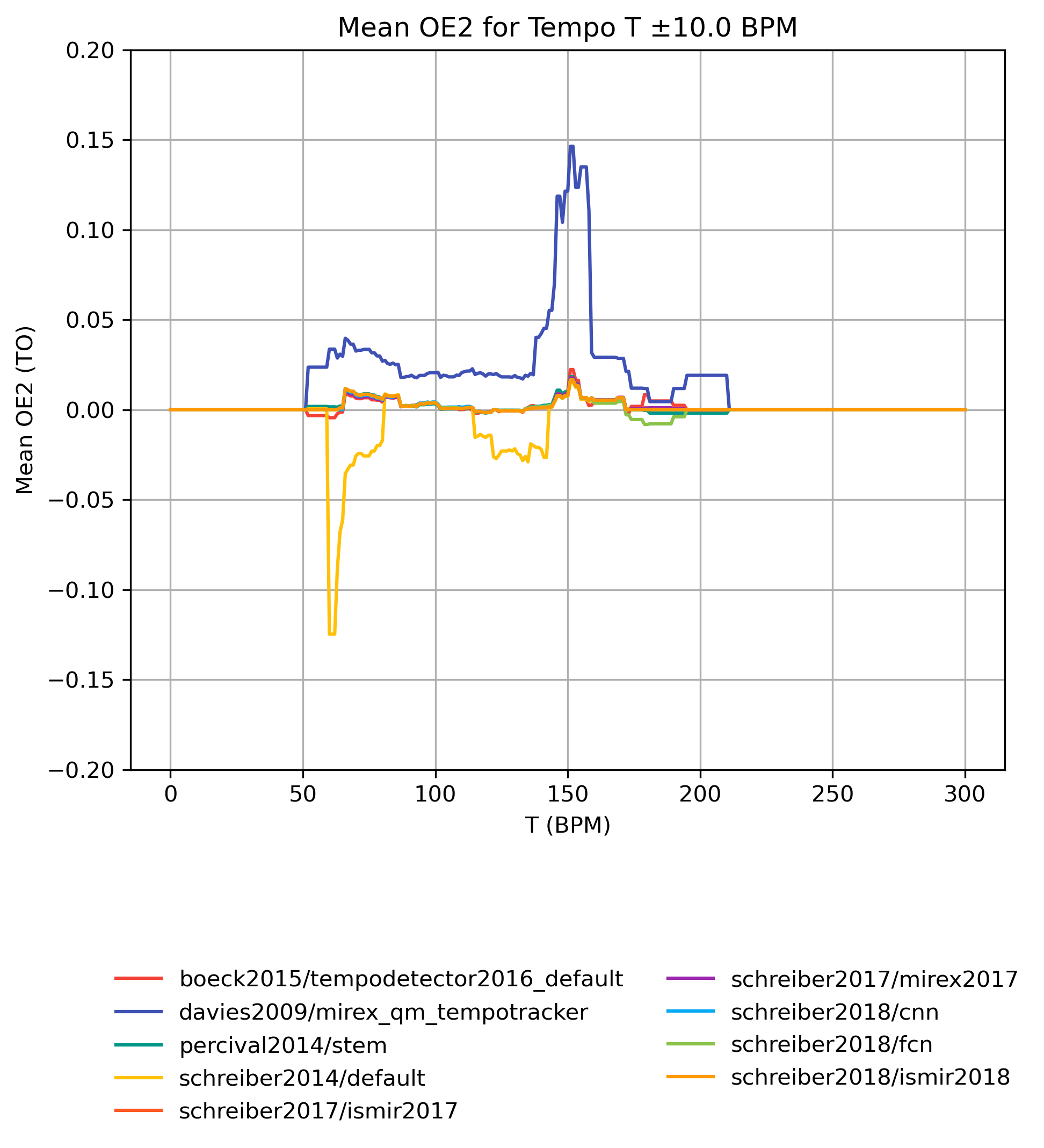
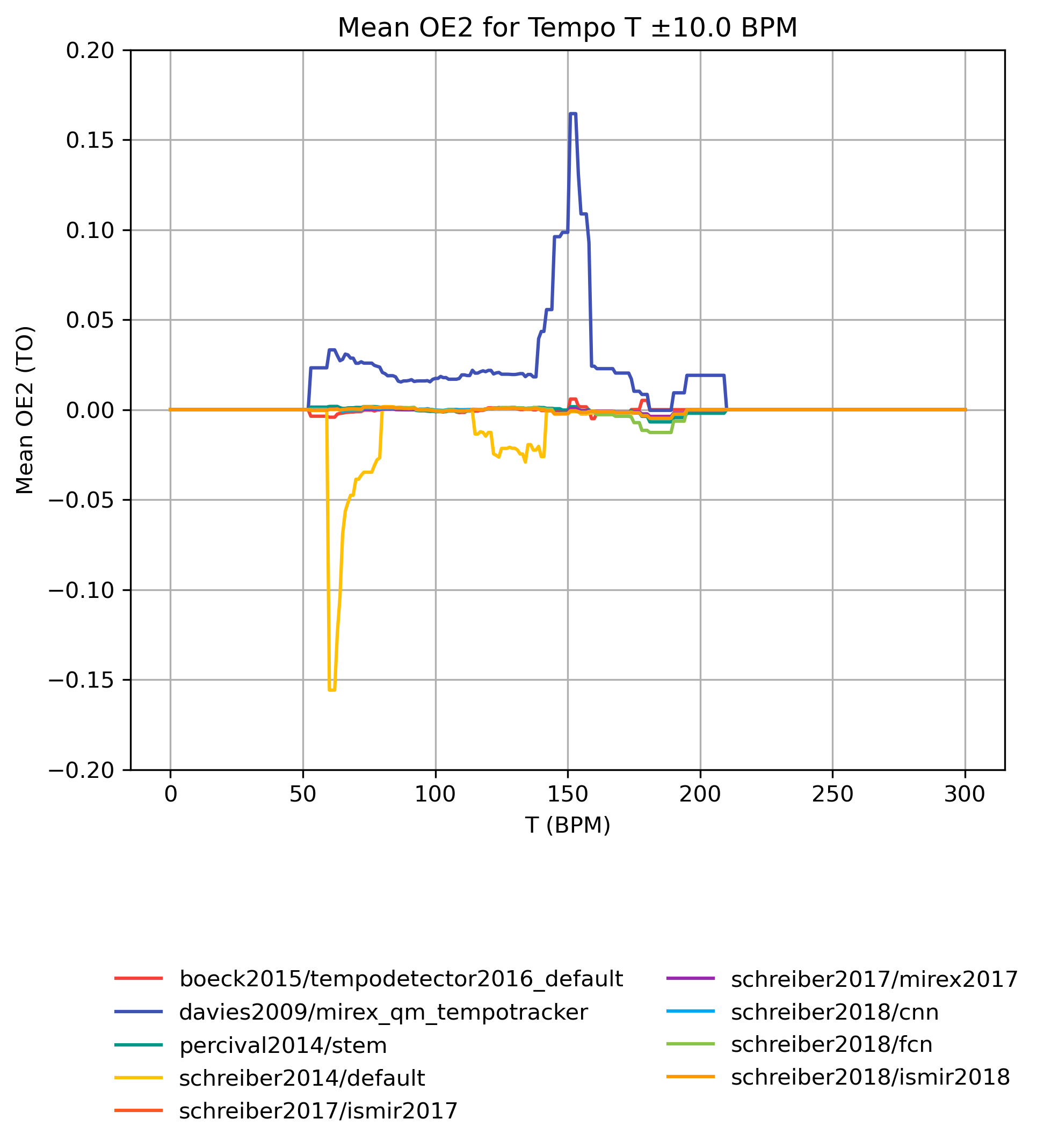
OE2 on Tempo-Subsets
How well does an estimator perform, when only taking a subset of the reference annotations into account? The graphs show mean OE2 for reference subsets with tempi in [T-10,T+10] BPM. Note that the graphs do not show confidence intervals and that some values may be based on very few estimates.
OE2 on Tempo-Subsets for 0.1
Figure 35: Mean OE2 for estimates compared to version 0.1 for tempo intervals around T.
CSV JSON LATEX PICKLE SVG PDF PNG
OE2 on Tempo-Subsets for 1.0
Figure 36: Mean OE2 for estimates compared to version 1.0 for tempo intervals around T.
CSV JSON LATEX PICKLE SVG PDF PNG
Estimated OE1 for Tempo
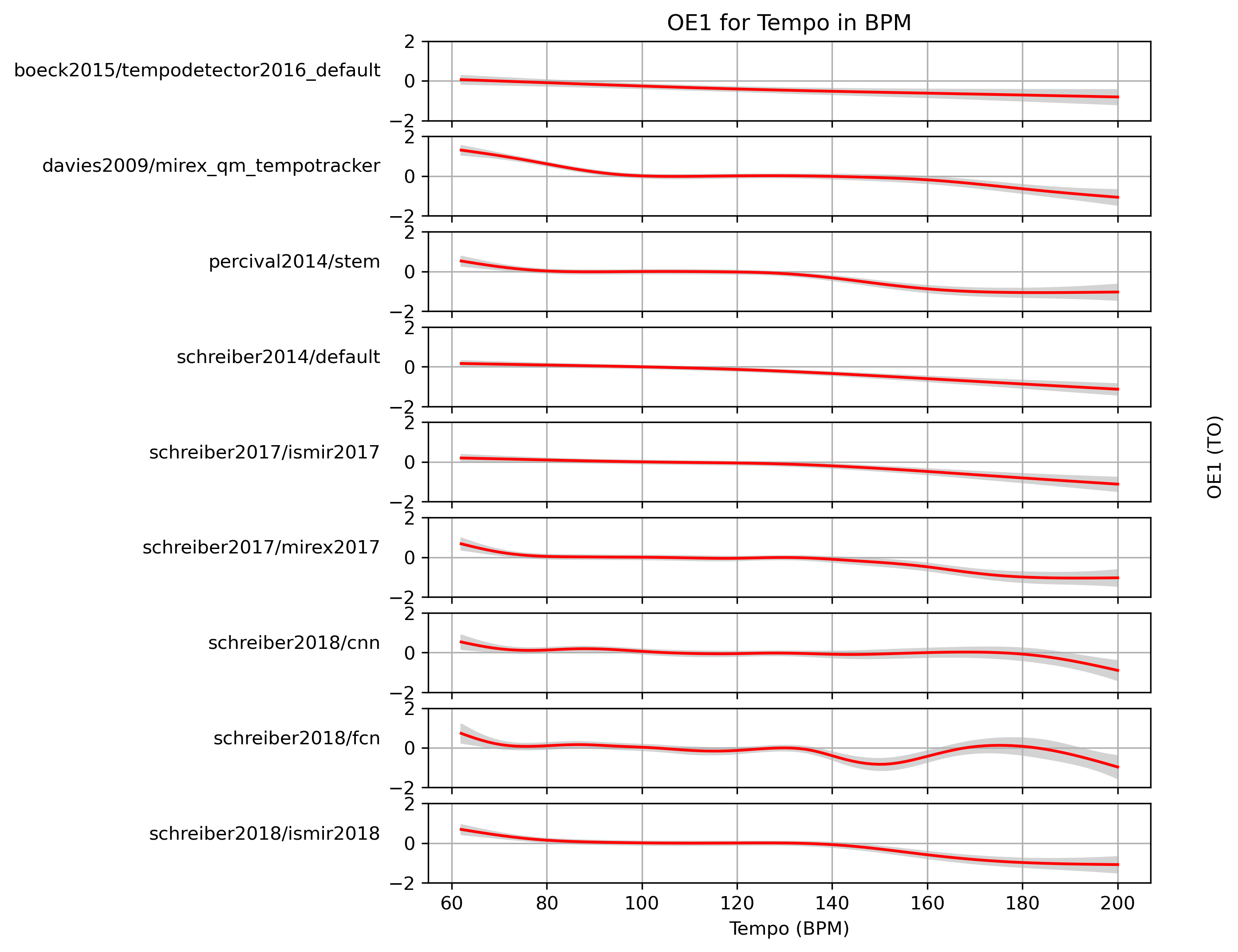
When fitting a generalized additive model (GAM) to OE1-values and a ground truth, what OE1 can we expect with confidence?
Estimated OE1 for Tempo for 0.1
Predictions of GAMs trained on OE1 for estimates for reference 0.1.
Figure 37: OE1 predictions of a generalized additive model (GAM) fit to OE1 results for 0.1. The 95% confidence interval around the prediction is shaded in gray.
CSV JSON LATEX PICKLE SVG PDF PNG
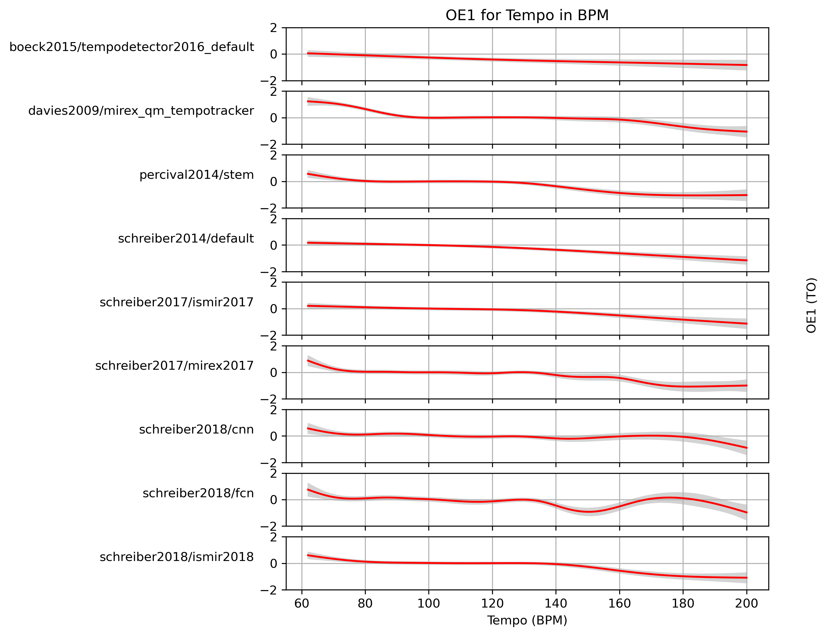
Estimated OE1 for Tempo for 1.0
Predictions of GAMs trained on OE1 for estimates for reference 1.0.
Figure 38: OE1 predictions of a generalized additive model (GAM) fit to OE1 results for 1.0. The 95% confidence interval around the prediction is shaded in gray.
CSV JSON LATEX PICKLE SVG PDF PNG
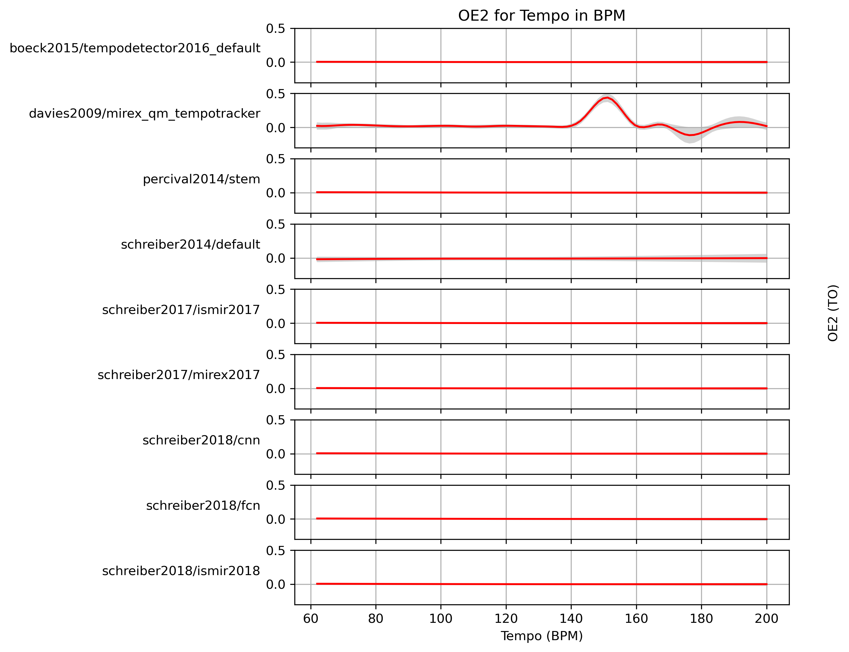
Estimated OE2 for Tempo
When fitting a generalized additive model (GAM) to OE2-values and a ground truth, what OE2 can we expect with confidence?
Estimated OE2 for Tempo for 0.1
Predictions of GAMs trained on OE2 for estimates for reference 0.1.
Figure 39: OE2 predictions of a generalized additive model (GAM) fit to OE2 results for 0.1. The 95% confidence interval around the prediction is shaded in gray.
CSV JSON LATEX PICKLE SVG PDF PNG
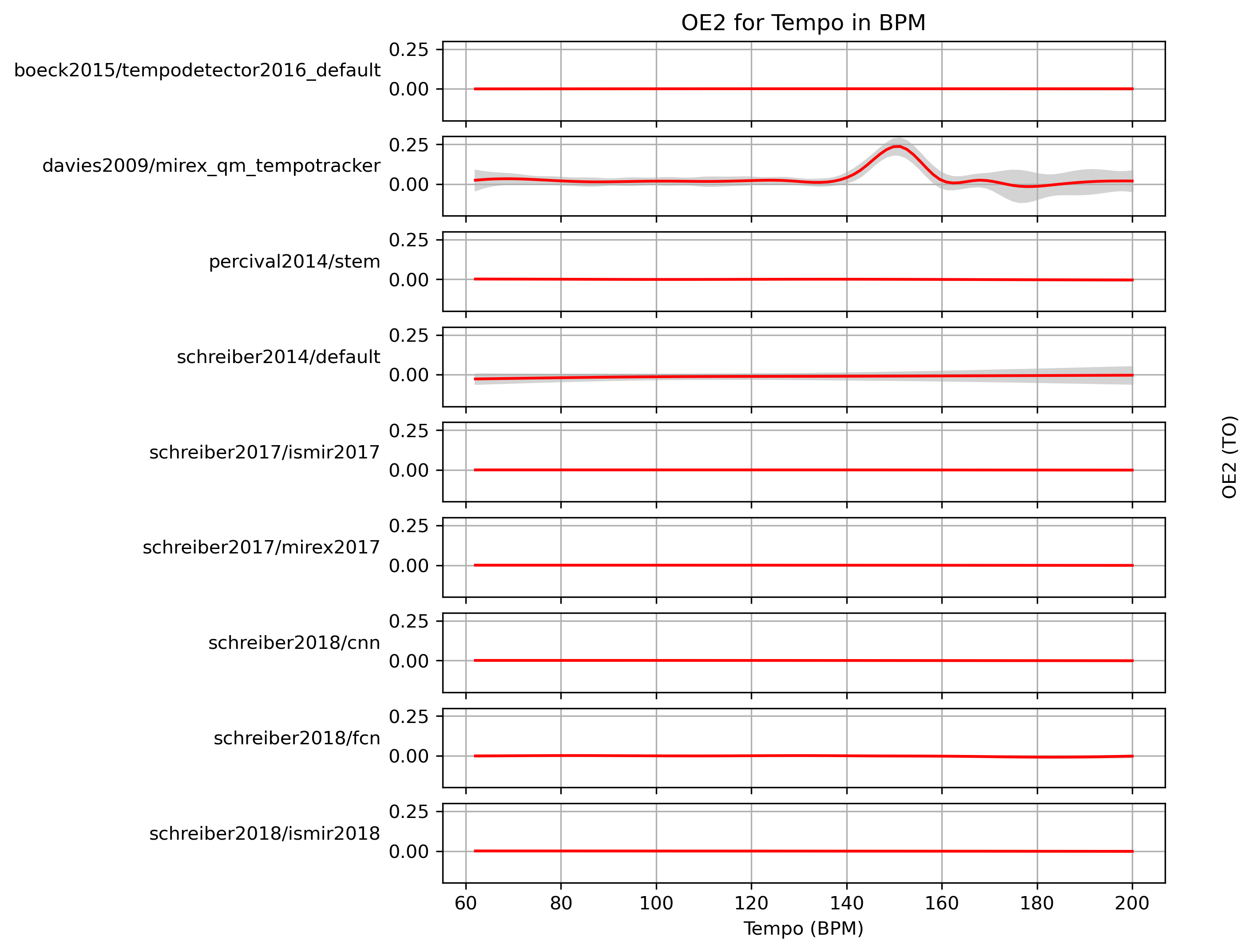
Estimated OE2 for Tempo for 1.0
Predictions of GAMs trained on OE2 for estimates for reference 1.0.
Figure 40: OE2 predictions of a generalized additive model (GAM) fit to OE2 results for 1.0. The 95% confidence interval around the prediction is shaded in gray.
CSV JSON LATEX PICKLE SVG PDF PNG
OE1 for ‘tag_open’ Tags
How well does an estimator perform, when only taking tracks into account that are tagged with some kind of label? Note that some values may be based on very few estimates.
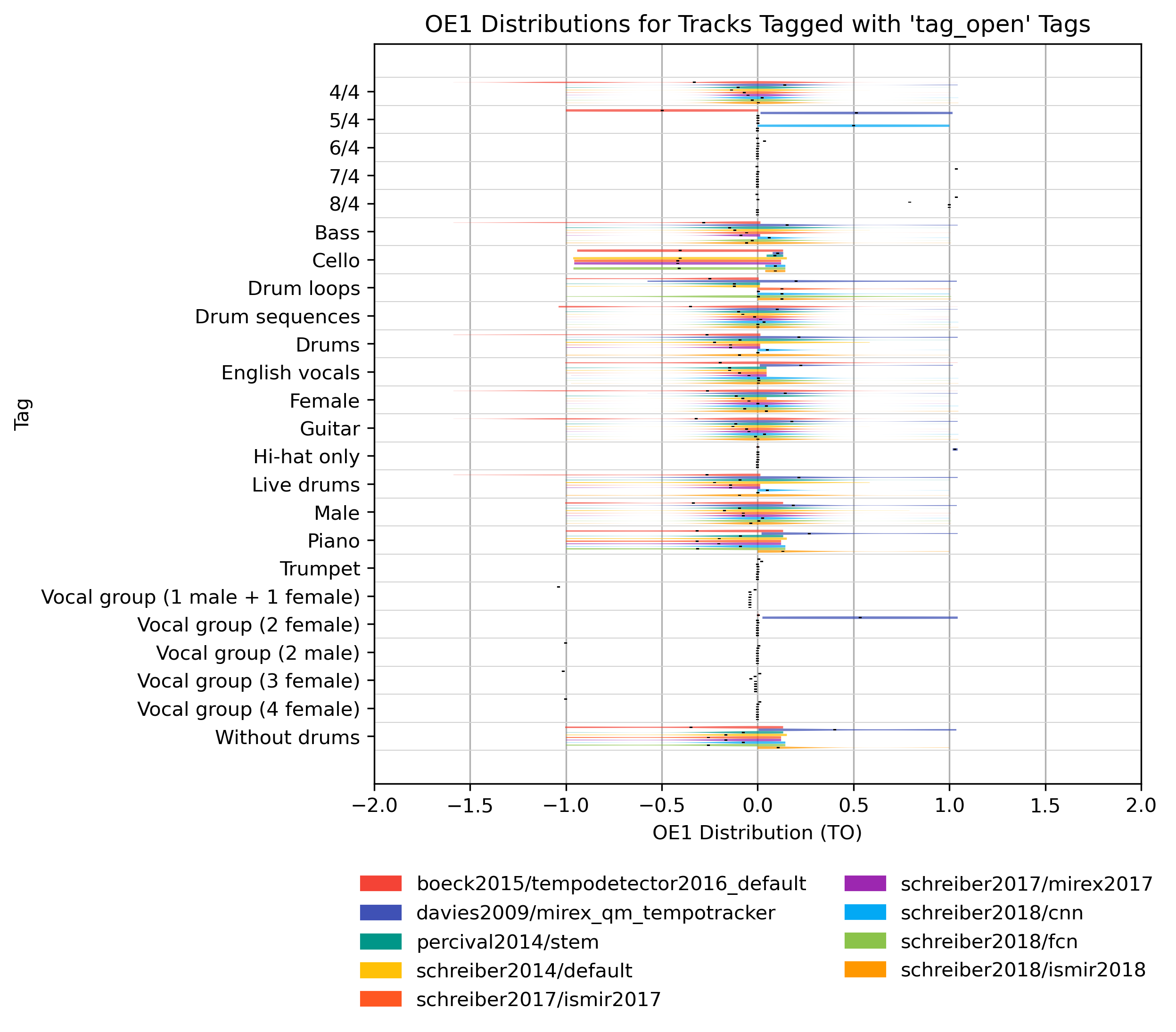
OE1 for ‘tag_open’ Tags for 0.1
Figure 41: OE1 of estimates compared to version 0.1 depending on tag from namespace ‘tag_open’.
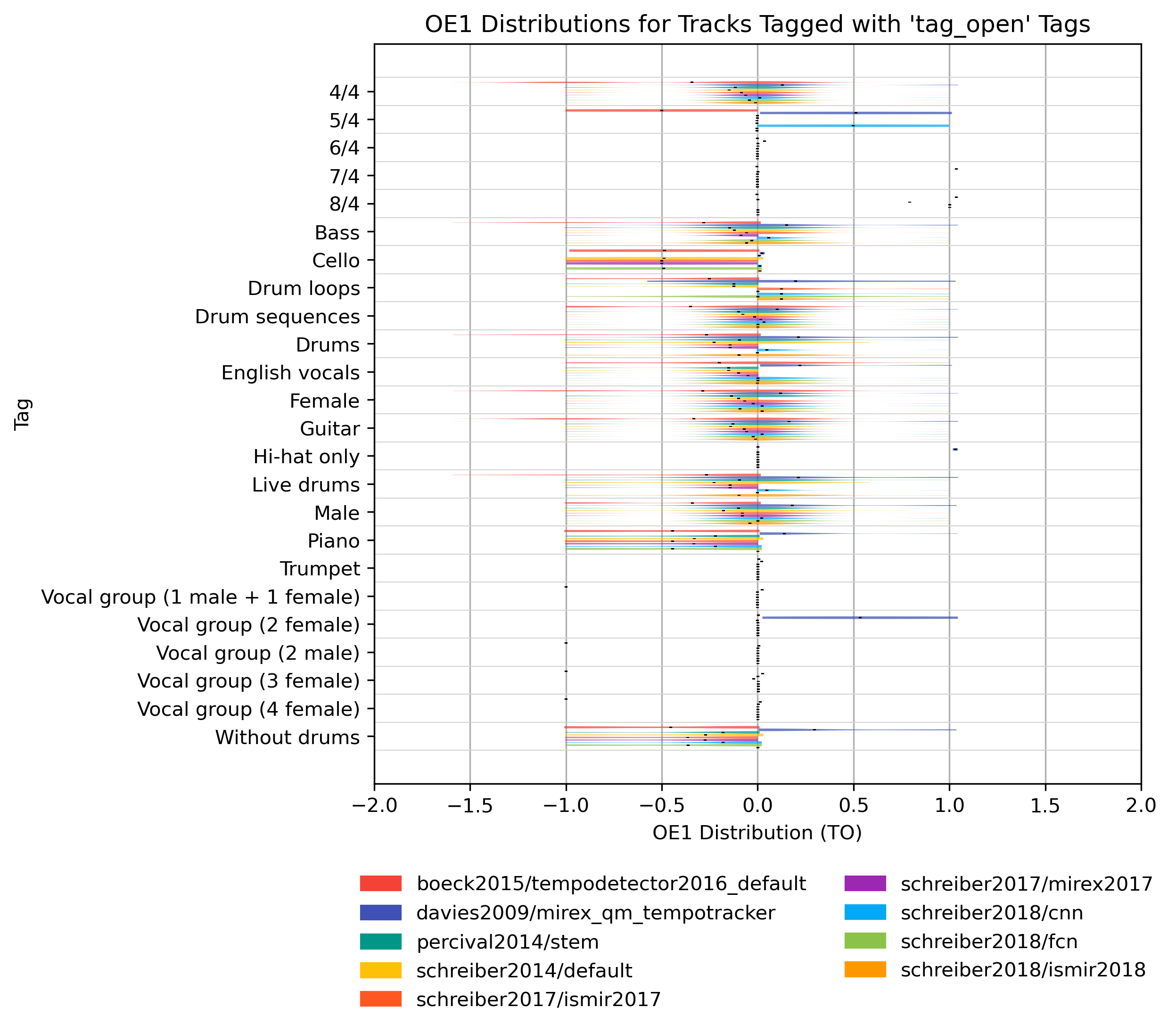
OE1 for ‘tag_open’ Tags for 1.0
Figure 42: OE1 of estimates compared to version 1.0 depending on tag from namespace ‘tag_open’.
OE2 for ‘tag_open’ Tags
How well does an estimator perform, when only taking tracks into account that are tagged with some kind of label? Note that some values may be based on very few estimates.
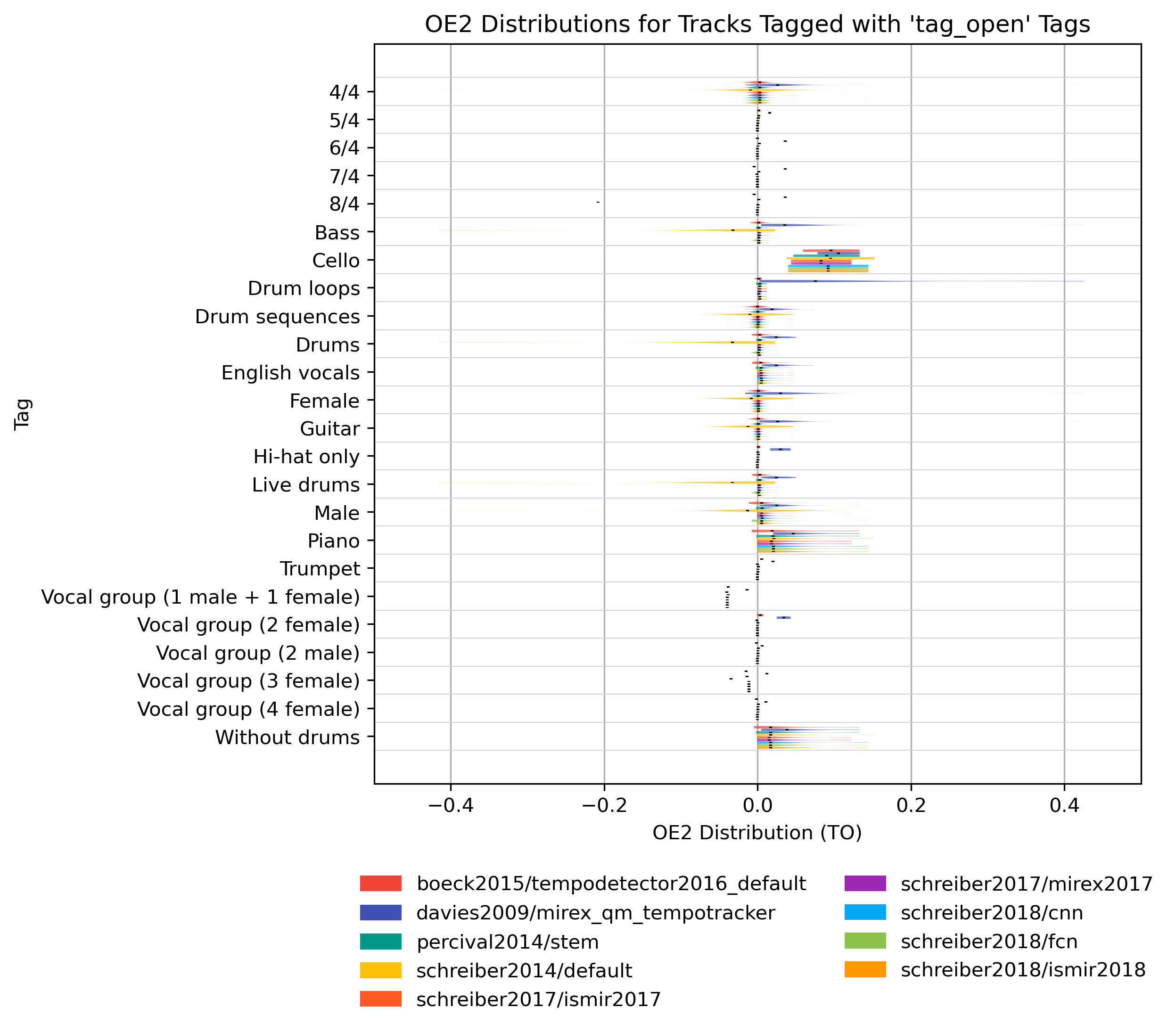
OE2 for ‘tag_open’ Tags for 0.1
Figure 43: OE2 of estimates compared to version 0.1 depending on tag from namespace ‘tag_open’.
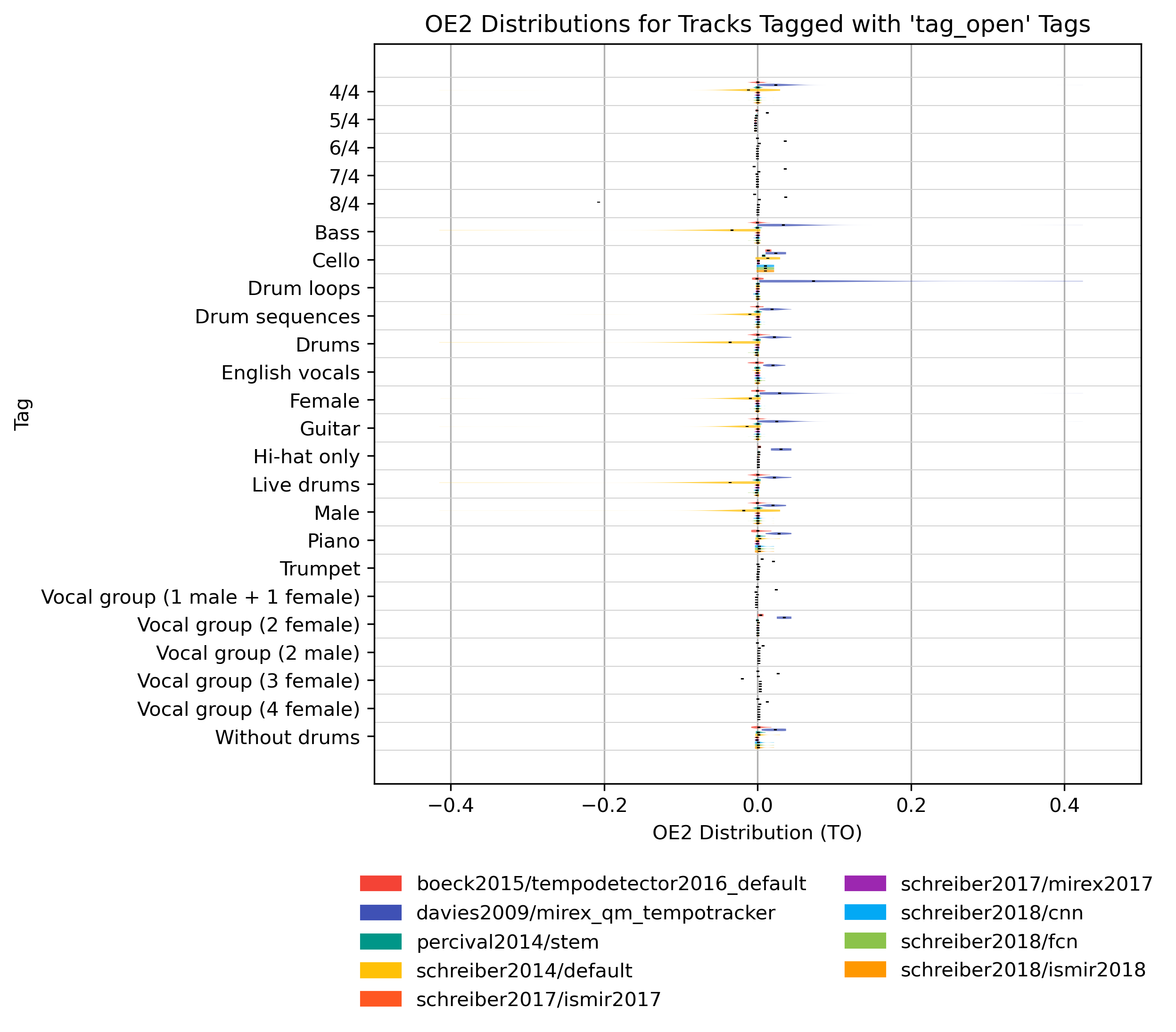
OE2 for ‘tag_open’ Tags for 1.0
Figure 44: OE2 of estimates compared to version 1.0 depending on tag from namespace ‘tag_open’.
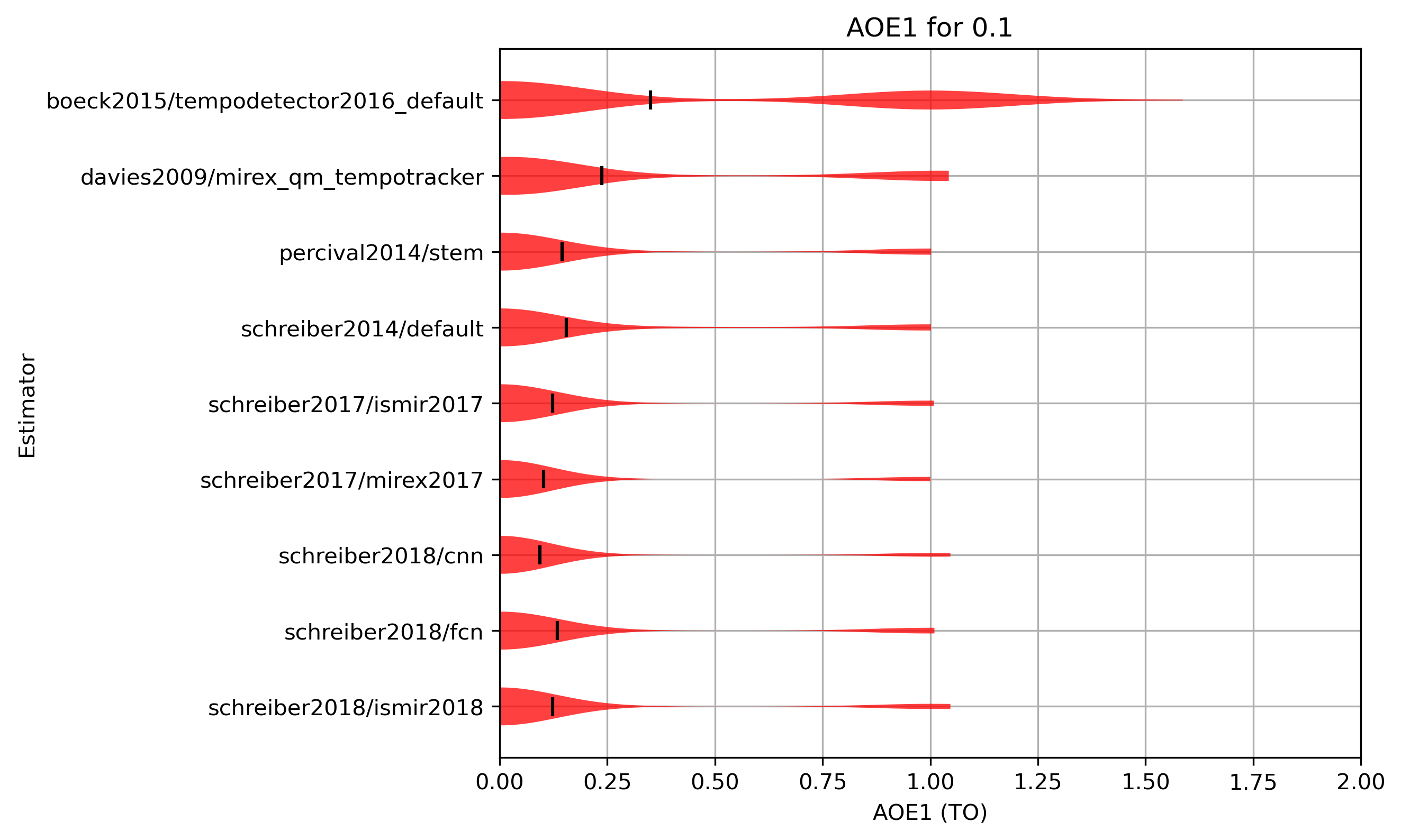
AOE1 and AOE2
AOE1 is defined as absolute octave error between an estimate and a reference value: AOE1(E) = |log2(E/R)|.
AOE2 is the minimum of AOE1 allowing the octave errors 2, 3, 1/2, and 1/3: AOE2(E) = min(AOE1(E), AOE1(2E), AOE1(3E), AOE1(½E), AOE1(⅓E)).
Mean AOE1/AOE2 Results for 0.1
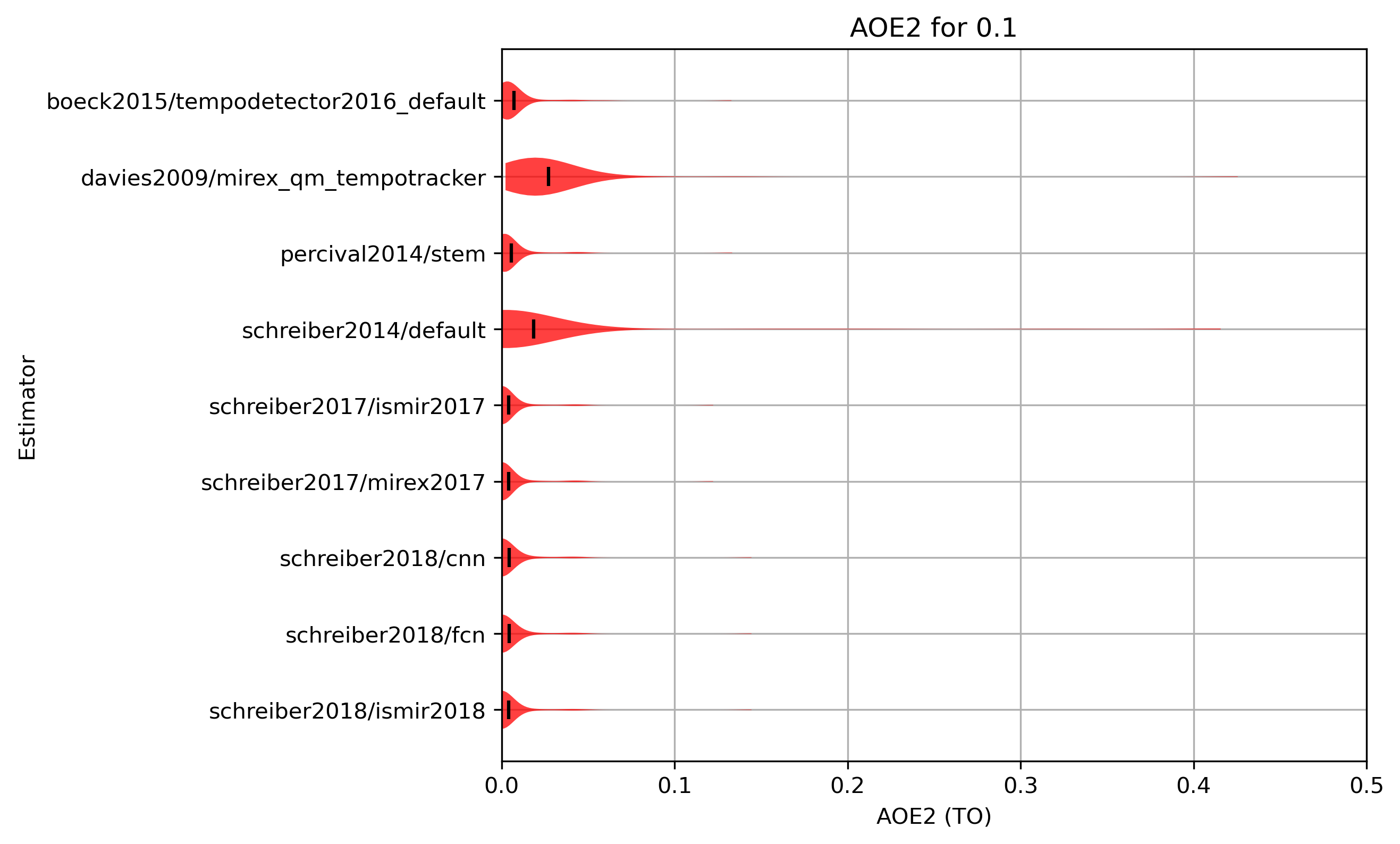
| Estimator | AOE1_MEAN | AOE1_STDEV | AOE2_MEAN | AOE2_STDEV |
|---|---|---|---|---|
| schreiber2018/cnn | 0.0942 | 0.2870 | 0.0042 | 0.0167 |
| schreiber2017/mirex2017 | 0.1027 | 0.2971 | 0.0041 | 0.0149 |
| schreiber2017/ismir2017 | 0.1227 | 0.3224 | 0.0041 | 0.0149 |
| schreiber2018/ismir2018 | 0.1235 | 0.3250 | 0.0041 | 0.0167 |
| schreiber2018/fcn | 0.1336 | 0.3347 | 0.0044 | 0.0167 |
| percival2014/stem | 0.1447 | 0.3448 | 0.0055 | 0.0157 |
| schreiber2014/default | 0.1546 | 0.3430 | 0.0184 | 0.0700 |
| davies2009/mirex_qm_tempotracker | 0.2379 | 0.4082 | 0.0271 | 0.0438 |
| boeck2015/tempodetector2016_default | 0.3505 | 0.4828 | 0.0070 | 0.0158 |
Table 15: Mean AOE1/AOE2 for estimates compared to version 0.1 ordered by mean.
Raw data AOE1: CSV JSON LATEX PICKLE
Raw data AOE2: CSV JSON LATEX PICKLE
AOE1 distribution for 0.1
Figure 45: AOE1 for estimates compared to version 0.1. Shown are the mean AOE1 and an empirical distribution of the sample, using kernel density estimation (KDE).
CSV JSON LATEX PICKLE SVG PDF PNG
AOE2 distribution for 0.1
Figure 46: AOE2 for estimates compared to version 0.1. Shown are the mean AOE2 and an empirical distribution of the sample, using kernel density estimation (KDE).
CSV JSON LATEX PICKLE SVG PDF PNG
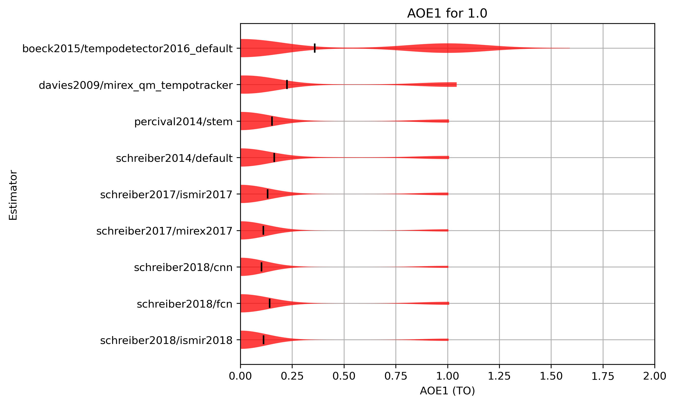
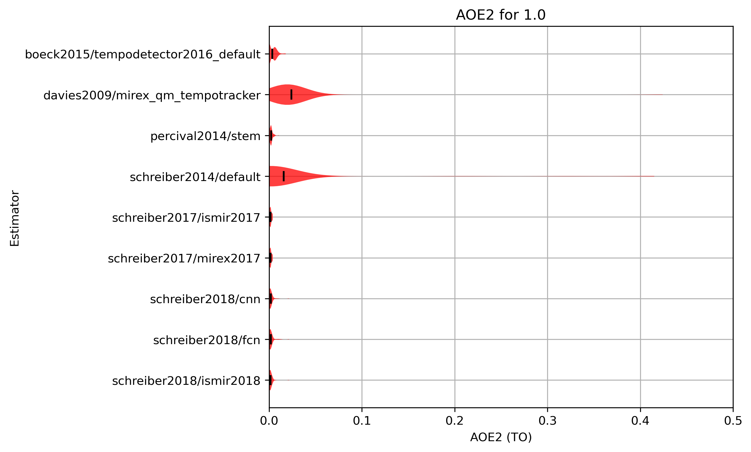
Mean AOE1/AOE2 Results for 1.0
| Estimator | AOE1_MEAN | AOE1_STDEV | AOE2_MEAN | AOE2_STDEV |
|---|---|---|---|---|
| schreiber2018/cnn | 0.1016 | 0.2993 | 0.0018 | 0.0025 |
| schreiber2017/mirex2017 | 0.1114 | 0.3126 | 0.0015 | 0.0011 |
| schreiber2018/ismir2018 | 0.1116 | 0.3126 | 0.0017 | 0.0024 |
| schreiber2017/ismir2017 | 0.1314 | 0.3362 | 0.0015 | 0.0011 |
| schreiber2018/fcn | 0.1419 | 0.3467 | 0.0020 | 0.0029 |
| percival2014/stem | 0.1521 | 0.3568 | 0.0022 | 0.0016 |
| schreiber2014/default | 0.1631 | 0.3555 | 0.0156 | 0.0683 |
| davies2009/mirex_qm_tempotracker | 0.2249 | 0.4018 | 0.0241 | 0.0415 |
| boeck2015/tempodetector2016_default | 0.3587 | 0.4861 | 0.0036 | 0.0040 |
Table 16: Mean AOE1/AOE2 for estimates compared to version 1.0 ordered by mean.
Raw data AOE1: CSV JSON LATEX PICKLE
Raw data AOE2: CSV JSON LATEX PICKLE
AOE1 distribution for 1.0
Figure 47: AOE1 for estimates compared to version 1.0. Shown are the mean AOE1 and an empirical distribution of the sample, using kernel density estimation (KDE).
CSV JSON LATEX PICKLE SVG PDF PNG
AOE2 distribution for 1.0
Figure 48: AOE2 for estimates compared to version 1.0. Shown are the mean AOE2 and an empirical distribution of the sample, using kernel density estimation (KDE).
CSV JSON LATEX PICKLE SVG PDF PNG
Significance of Differences
| Estimator | boeck2015/tempodetector2016_default | davies2009/mirex_qm_tempotracker | percival2014/stem | schreiber2014/default | schreiber2017/ismir2017 | schreiber2017/mirex2017 | schreiber2018/cnn | schreiber2018/fcn | schreiber2018/ismir2018 |
|---|---|---|---|---|---|---|---|---|---|
| boeck2015/tempodetector2016_default | 1.0000 | 0.0612 | 0.0005 | 0.0002 | 0.0001 | 0.0000 | 0.0000 | 0.0002 | 0.0000 |
| davies2009/mirex_qm_tempotracker | 0.0612 | 1.0000 | 0.1416 | 0.2366 | 0.0437 | 0.0099 | 0.0090 | 0.0997 | 0.0066 |
| percival2014/stem | 0.0005 | 0.1416 | 1.0000 | 0.7316 | 0.5534 | 0.1995 | 0.1933 | 0.7949 | 0.2019 |
| schreiber2014/default | 0.0002 | 0.2366 | 0.7316 | 1.0000 | 0.2832 | 0.0785 | 0.1389 | 0.6315 | 0.1858 |
| schreiber2017/ismir2017 | 0.0001 | 0.0437 | 0.5534 | 0.2832 | 1.0000 | 0.3195 | 0.4106 | 0.7714 | 0.5333 |
| schreiber2017/mirex2017 | 0.0000 | 0.0099 | 0.1995 | 0.0785 | 0.3195 | 1.0000 | 0.7872 | 0.4324 | 0.9944 |
| schreiber2018/cnn | 0.0000 | 0.0090 | 0.1933 | 0.1389 | 0.4106 | 0.7872 | 1.0000 | 0.1545 | 0.7832 |
| schreiber2018/fcn | 0.0002 | 0.0997 | 0.7949 | 0.6315 | 0.7714 | 0.4324 | 0.1545 | 1.0000 | 0.4639 |
| schreiber2018/ismir2018 | 0.0000 | 0.0066 | 0.2019 | 0.1858 | 0.5333 | 0.9944 | 0.7832 | 0.4639 | 1.0000 |
Table 17: Paired t-test p-values, using reference annotations 1.0 as groundtruth with AOE1. H0: the true mean difference between paired samples is zero. If p<=ɑ, reject H0, i.e. we have a significant difference between estimates from the two algorithms. In the table, p-values<0.05 are set in bold.
| Estimator | boeck2015/tempodetector2016_default | davies2009/mirex_qm_tempotracker | percival2014/stem | schreiber2014/default | schreiber2017/ismir2017 | schreiber2017/mirex2017 | schreiber2018/cnn | schreiber2018/fcn | schreiber2018/ismir2018 |
|---|---|---|---|---|---|---|---|---|---|
| boeck2015/tempodetector2016_default | 1.0000 | 0.1159 | 0.0006 | 0.0002 | 0.0001 | 0.0000 | 0.0000 | 0.0002 | 0.0002 |
| davies2009/mirex_qm_tempotracker | 0.1159 | 1.0000 | 0.0596 | 0.1092 | 0.0122 | 0.0019 | 0.0023 | 0.0380 | 0.0060 |
| percival2014/stem | 0.0006 | 0.0596 | 1.0000 | 0.7574 | 0.5238 | 0.1809 | 0.1913 | 0.7731 | 0.5049 |
| schreiber2014/default | 0.0002 | 0.1092 | 0.7574 | 1.0000 | 0.2798 | 0.0774 | 0.1434 | 0.6333 | 0.4237 |
| schreiber2017/ismir2017 | 0.0001 | 0.0122 | 0.5238 | 0.2798 | 1.0000 | 0.3198 | 0.4277 | 0.7621 | 0.9785 |
| schreiber2017/mirex2017 | 0.0000 | 0.0019 | 0.1809 | 0.0774 | 0.3198 | 1.0000 | 0.8136 | 0.4252 | 0.4593 |
| schreiber2018/cnn | 0.0000 | 0.0023 | 0.1913 | 0.1434 | 0.4277 | 0.8136 | 1.0000 | 0.1610 | 0.4170 |
| schreiber2018/fcn | 0.0002 | 0.0380 | 0.7731 | 0.6333 | 0.7621 | 0.4252 | 0.1610 | 1.0000 | 0.8066 |
| schreiber2018/ismir2018 | 0.0002 | 0.0060 | 0.5049 | 0.4237 | 0.9785 | 0.4593 | 0.4170 | 0.8066 | 1.0000 |
Table 18: Paired t-test p-values, using reference annotations 0.1 as groundtruth with AOE1. H0: the true mean difference between paired samples is zero. If p<=ɑ, reject H0, i.e. we have a significant difference between estimates from the two algorithms. In the table, p-values<0.05 are set in bold.
| Estimator | boeck2015/tempodetector2016_default | davies2009/mirex_qm_tempotracker | percival2014/stem | schreiber2014/default | schreiber2017/ismir2017 | schreiber2017/mirex2017 | schreiber2018/cnn | schreiber2018/fcn | schreiber2018/ismir2018 |
|---|---|---|---|---|---|---|---|---|---|
| boeck2015/tempodetector2016_default | 1.0000 | 0.0000 | 0.0015 | 0.0848 | 0.0000 | 0.0000 | 0.0001 | 0.0007 | 0.0000 |
| davies2009/mirex_qm_tempotracker | 0.0000 | 1.0000 | 0.0000 | 0.2957 | 0.0000 | 0.0000 | 0.0000 | 0.0000 | 0.0000 |
| percival2014/stem | 0.0015 | 0.0000 | 1.0000 | 0.0534 | 0.0001 | 0.0001 | 0.1158 | 0.5593 | 0.0199 |
| schreiber2014/default | 0.0848 | 0.2957 | 0.0534 | 1.0000 | 0.0430 | 0.0430 | 0.0483 | 0.0518 | 0.0462 |
| schreiber2017/ismir2017 | 0.0000 | 0.0000 | 0.0001 | 0.0430 | 1.0000 | 0.2449 | 0.1780 | 0.0565 | 0.3624 |
| schreiber2017/mirex2017 | 0.0000 | 0.0000 | 0.0001 | 0.0430 | 0.2449 | 1.0000 | 0.1780 | 0.0565 | 0.3624 |
| schreiber2018/cnn | 0.0001 | 0.0000 | 0.1158 | 0.0483 | 0.1780 | 0.1780 | 1.0000 | 0.1481 | 0.1829 |
| schreiber2018/fcn | 0.0007 | 0.0000 | 0.5593 | 0.0518 | 0.0565 | 0.0565 | 0.1481 | 1.0000 | 0.0456 |
| schreiber2018/ismir2018 | 0.0000 | 0.0000 | 0.0199 | 0.0462 | 0.3624 | 0.3624 | 0.1829 | 0.0456 | 1.0000 |
Table 19: Paired t-test p-values, using reference annotations 1.0 as groundtruth with AOE2. H0: the true mean difference between paired samples is zero. If p<=ɑ, reject H0, i.e. we have a significant difference between estimates from the two algorithms. In the table, p-values<0.05 are set in bold.
| Estimator | boeck2015/tempodetector2016_default | davies2009/mirex_qm_tempotracker | percival2014/stem | schreiber2014/default | schreiber2017/ismir2017 | schreiber2017/mirex2017 | schreiber2018/cnn | schreiber2018/fcn | schreiber2018/ismir2018 |
|---|---|---|---|---|---|---|---|---|---|
| boeck2015/tempodetector2016_default | 1.0000 | 0.0000 | 0.0000 | 0.1049 | 0.0000 | 0.0000 | 0.0000 | 0.0000 | 0.0000 |
| davies2009/mirex_qm_tempotracker | 0.0000 | 1.0000 | 0.0000 | 0.2862 | 0.0000 | 0.0000 | 0.0000 | 0.0000 | 0.0000 |
| percival2014/stem | 0.0000 | 0.0000 | 1.0000 | 0.0640 | 0.0000 | 0.0000 | 0.0000 | 0.0000 | 0.0000 |
| schreiber2014/default | 0.1049 | 0.2862 | 0.0640 | 1.0000 | 0.0417 | 0.0417 | 0.0429 | 0.0460 | 0.0407 |
| schreiber2017/ismir2017 | 0.0000 | 0.0000 | 0.0000 | 0.0417 | 1.0000 | 0.4277 | 0.7770 | 0.3384 | 0.7668 |
| schreiber2017/mirex2017 | 0.0000 | 0.0000 | 0.0000 | 0.0417 | 0.4277 | 1.0000 | 0.7770 | 0.3384 | 0.7669 |
| schreiber2018/cnn | 0.0000 | 0.0000 | 0.0000 | 0.0429 | 0.7770 | 0.7770 | 1.0000 | 0.3747 | 0.4596 |
| schreiber2018/fcn | 0.0000 | 0.0000 | 0.0000 | 0.0460 | 0.3384 | 0.3384 | 0.3747 | 1.0000 | 0.0474 |
| schreiber2018/ismir2018 | 0.0000 | 0.0000 | 0.0000 | 0.0407 | 0.7668 | 0.7669 | 0.4596 | 0.0474 | 1.0000 |
Table 20: Paired t-test p-values, using reference annotations 0.1 as groundtruth with AOE2. H0: the true mean difference between paired samples is zero. If p<=ɑ, reject H0, i.e. we have a significant difference between estimates from the two algorithms. In the table, p-values<0.05 are set in bold.
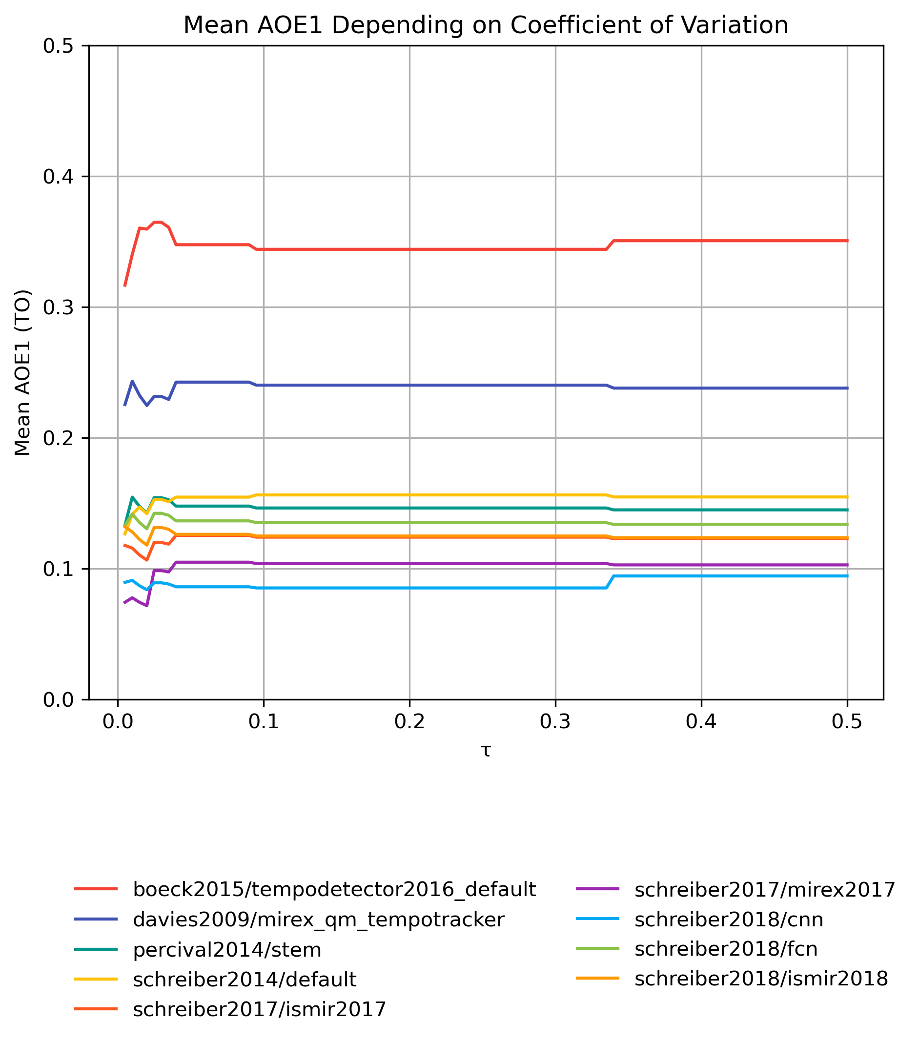
AOE1 on cvar-Subsets
How well does an estimator perform, when only taking tracks into account that have a cvar-value of less than τ, i.e., have a more or less stable beat?
AOE1 on cvar-Subsets for 0.1 based on cvar-Values from 1.0
Figure 49: Mean AOE1 compared to version 0.1 for tracks with cvar < τ based on beat annotations from 0.1.
CSV JSON LATEX PICKLE SVG PDF PNG
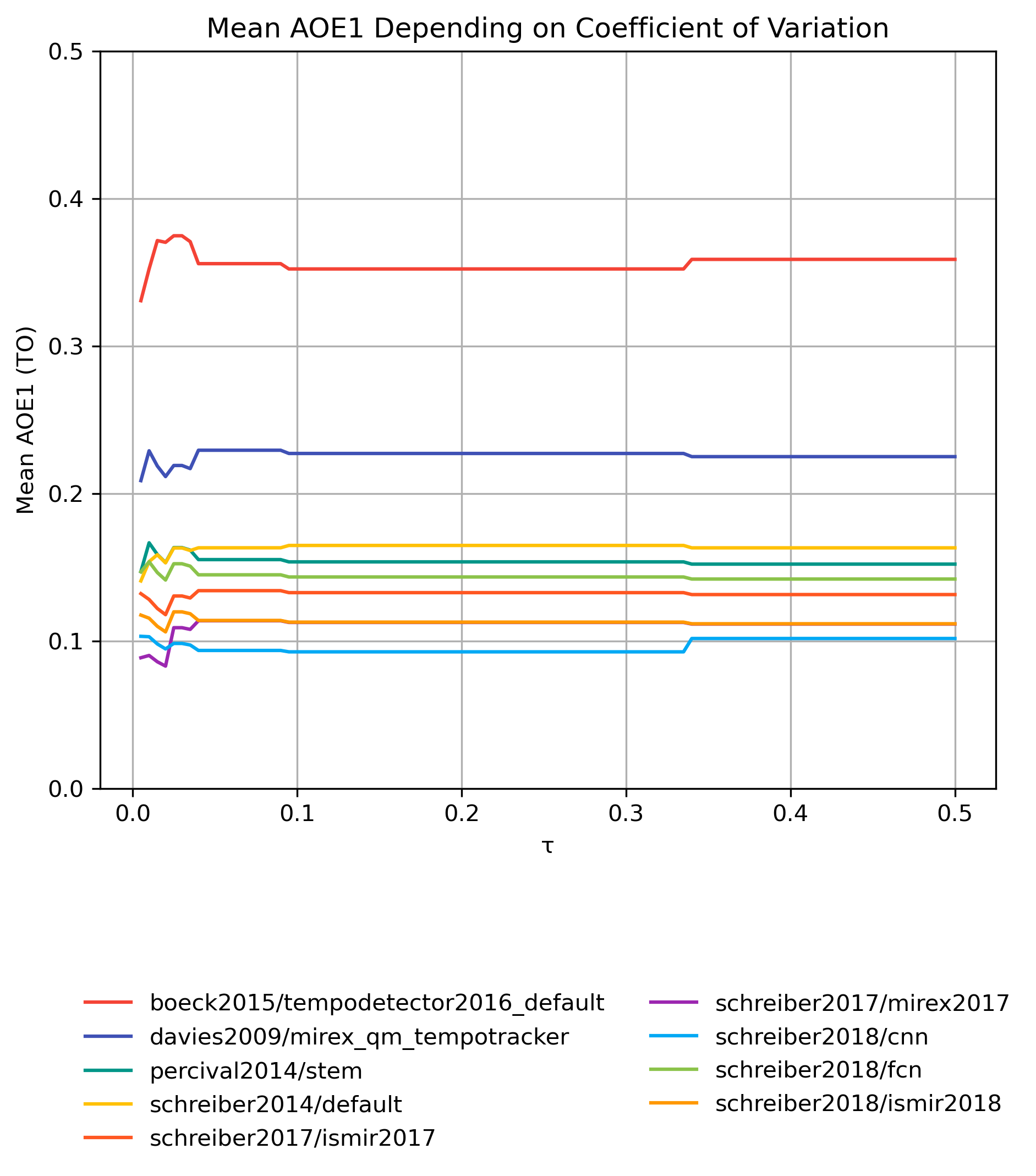
AOE1 on cvar-Subsets for 1.0 based on cvar-Values from 1.0
Figure 50: Mean AOE1 compared to version 1.0 for tracks with cvar < τ based on beat annotations from 1.0.
CSV JSON LATEX PICKLE SVG PDF PNG
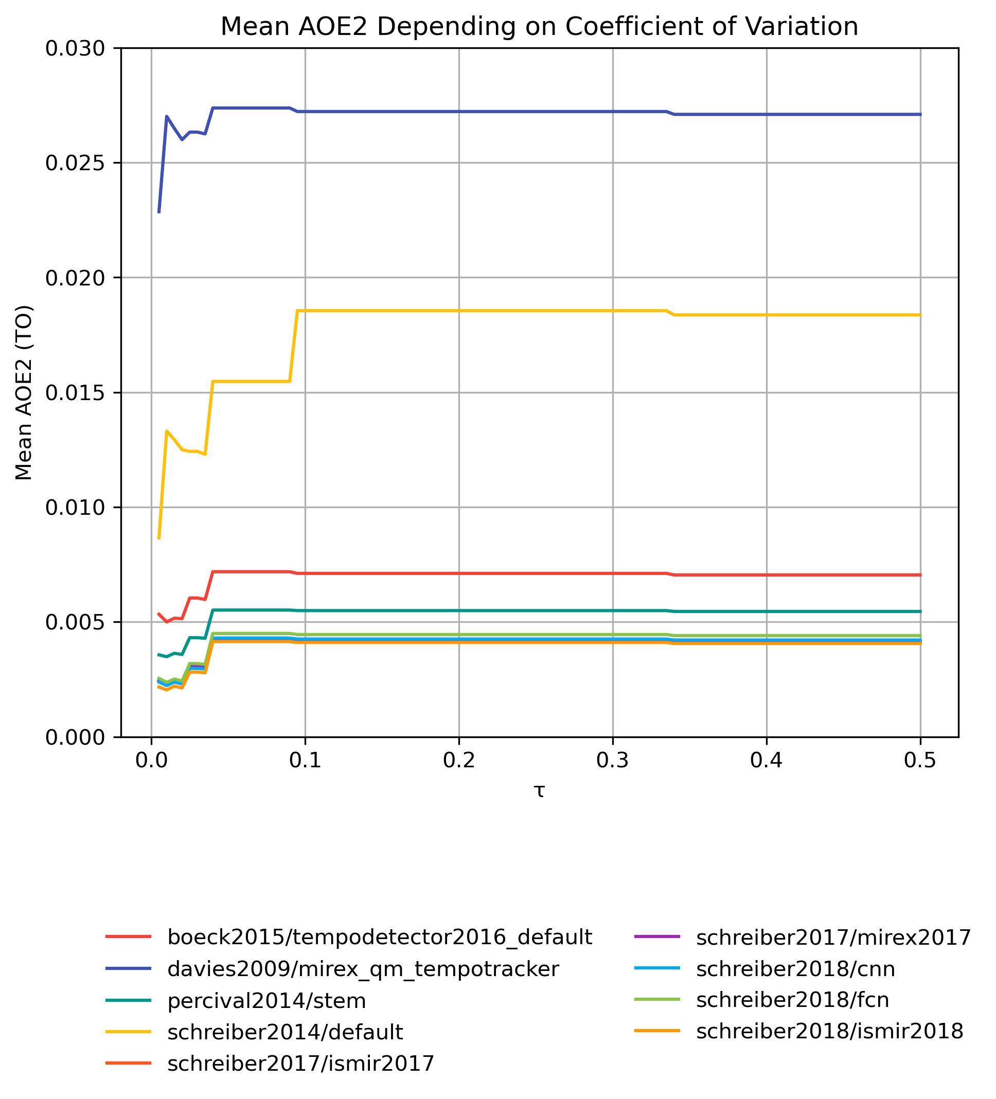
AOE2 on cvar-Subsets
How well does an estimator perform, when only taking tracks into account that have a cvar-value of less than τ, i.e., have a more or less stable beat?
AOE2 on cvar-Subsets for 0.1 based on cvar-Values from 1.0
Figure 51: Mean AOE2 compared to version 0.1 for tracks with cvar < τ based on beat annotations from 0.1.
CSV JSON LATEX PICKLE SVG PDF PNG
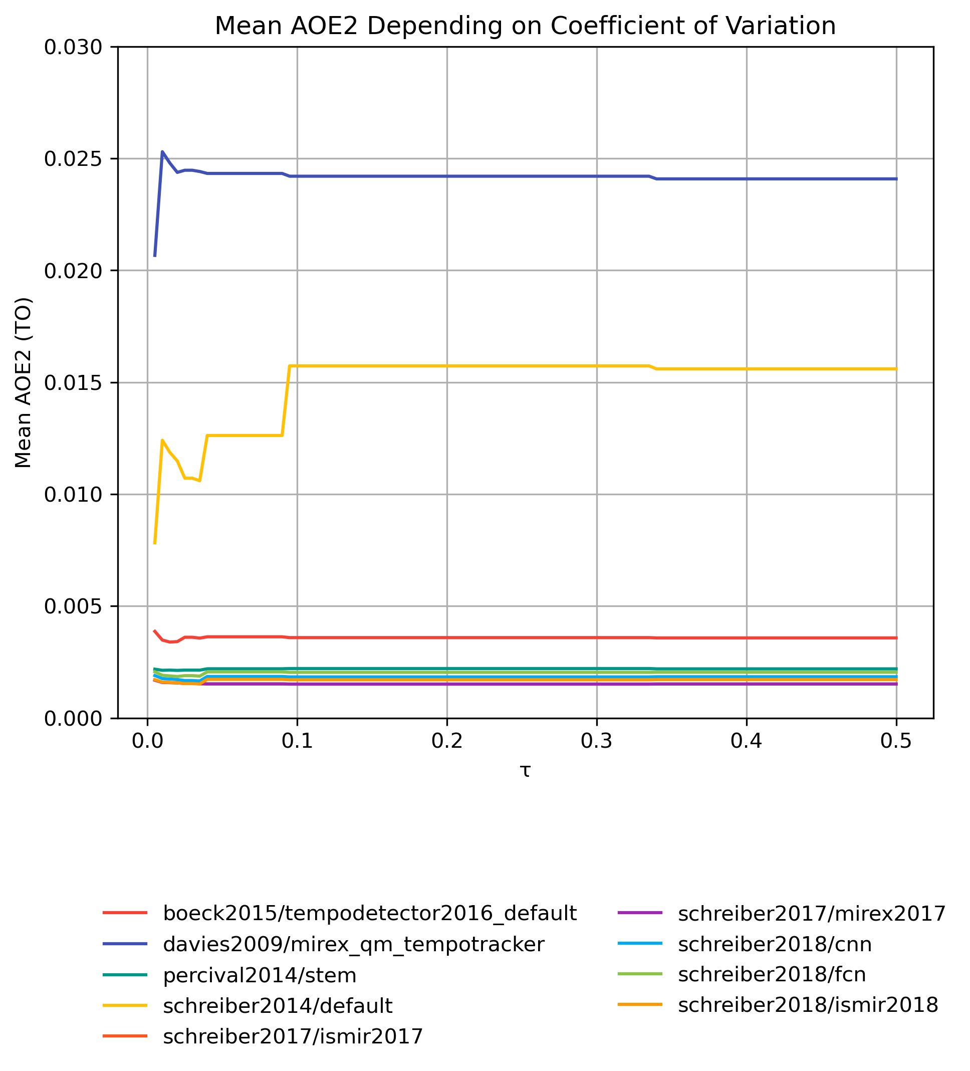
AOE2 on cvar-Subsets for 1.0 based on cvar-Values from 1.0
Figure 52: Mean AOE2 compared to version 1.0 for tracks with cvar < τ based on beat annotations from 1.0.
CSV JSON LATEX PICKLE SVG PDF PNG
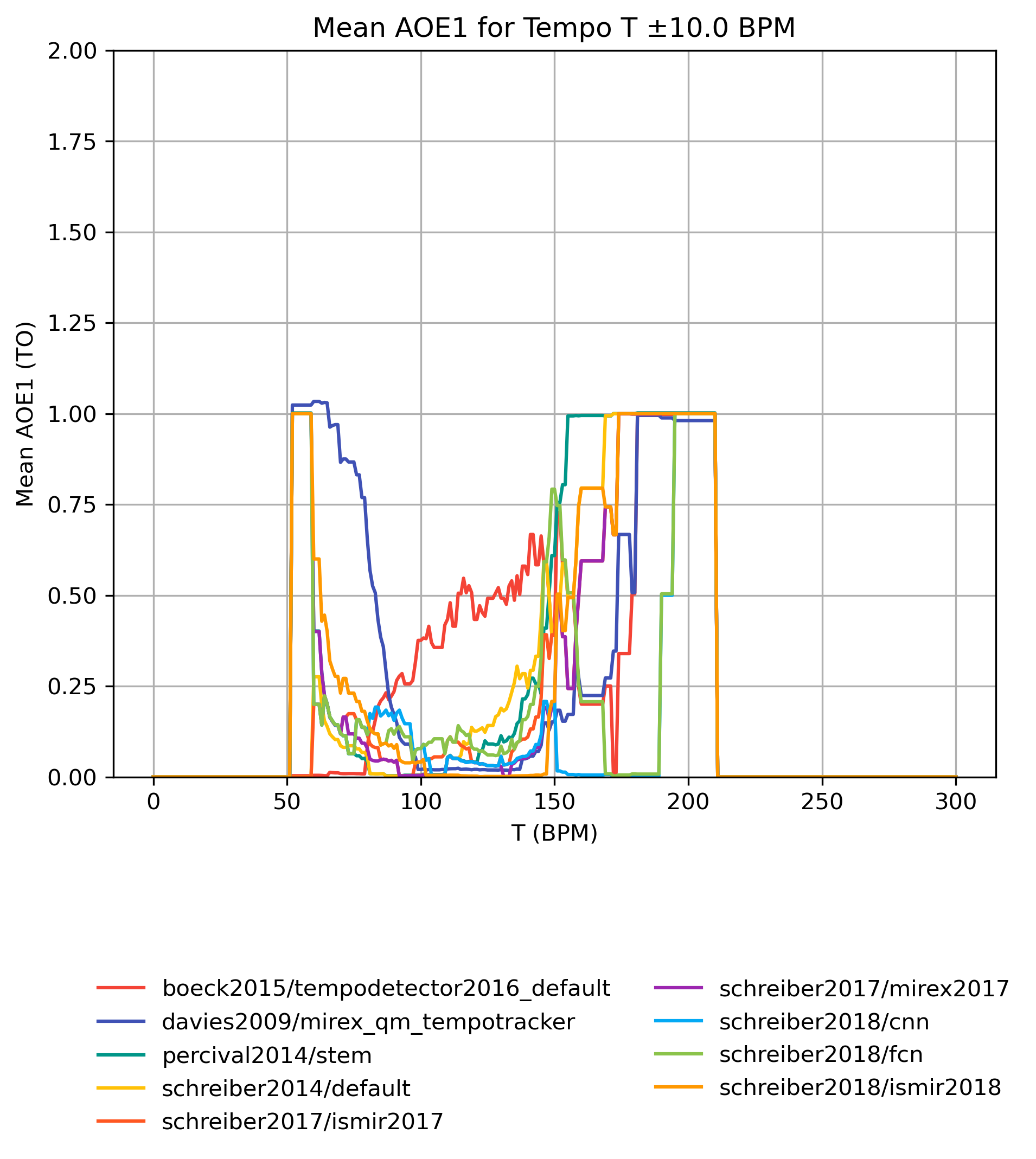
AOE1 on Tempo-Subsets
How well does an estimator perform, when only taking a subset of the reference annotations into account? The graphs show mean AOE1 for reference subsets with tempi in [T-10,T+10] BPM. Note that the graphs do not show confidence intervals and that some values may be based on very few estimates.
AOE1 on Tempo-Subsets for 0.1
Figure 53: Mean AOE1 for estimates compared to version 0.1 for tempo intervals around T.
CSV JSON LATEX PICKLE SVG PDF PNG
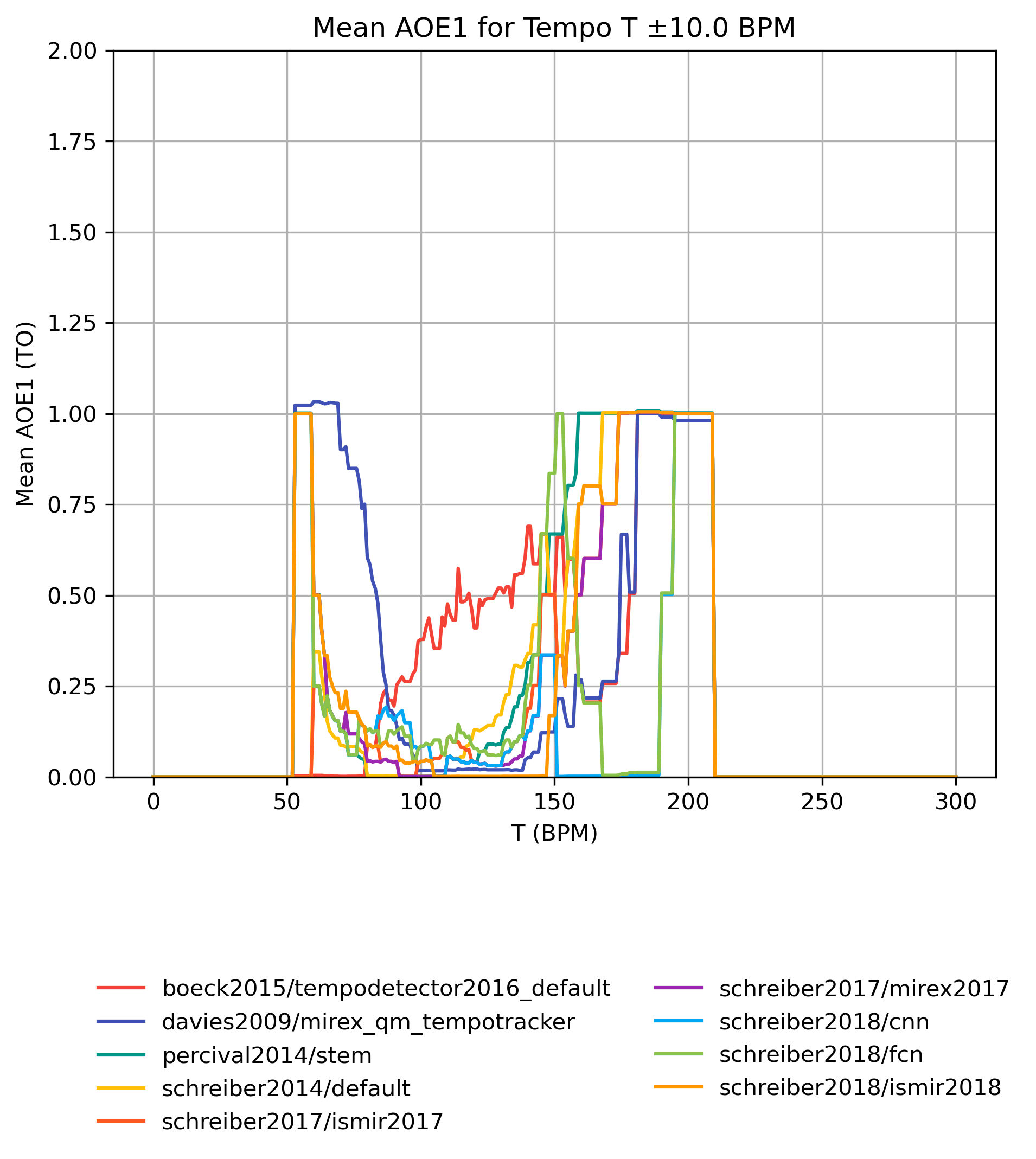
AOE1 on Tempo-Subsets for 1.0
Figure 54: Mean AOE1 for estimates compared to version 1.0 for tempo intervals around T.
CSV JSON LATEX PICKLE SVG PDF PNG
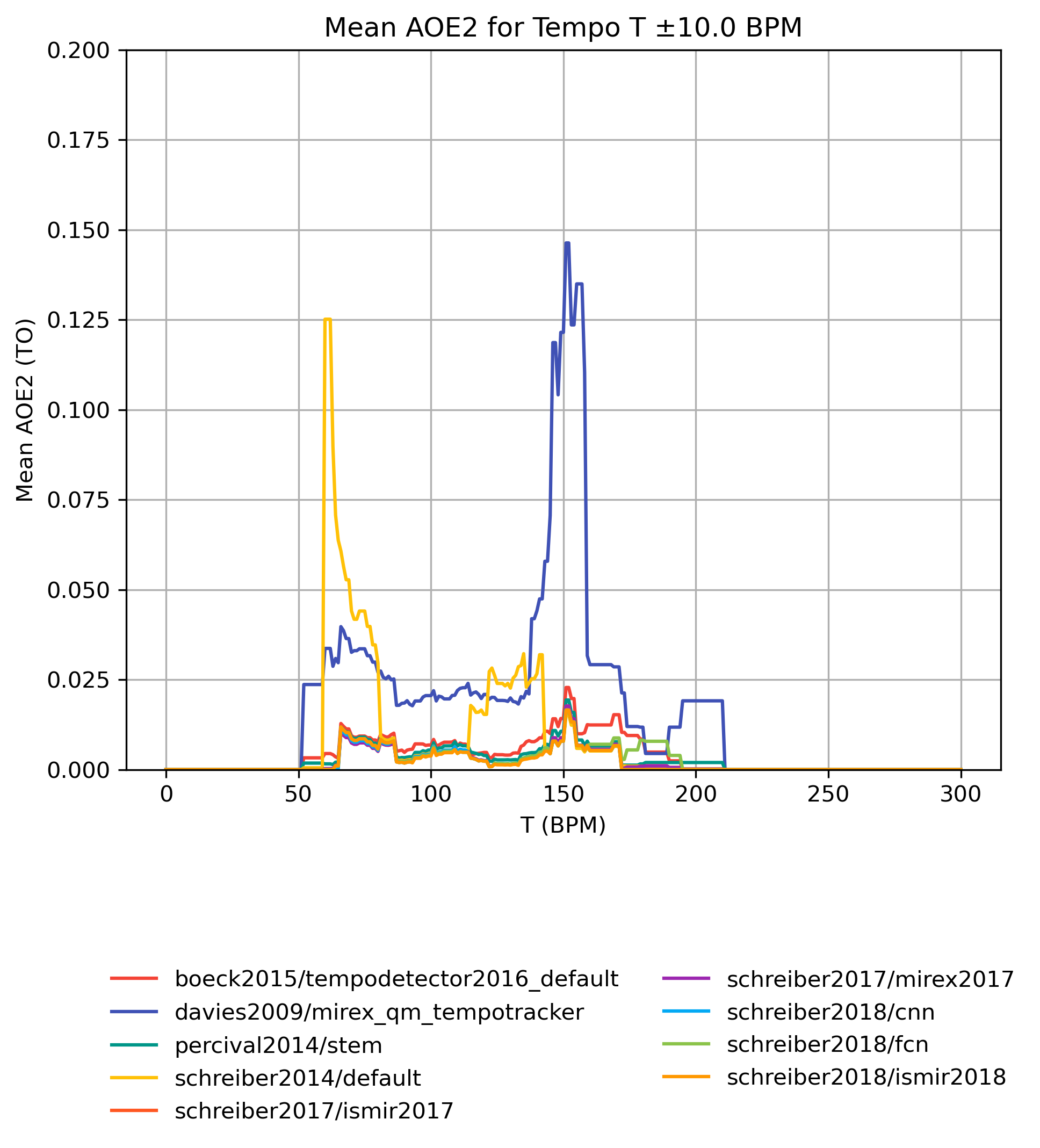
AOE2 on Tempo-Subsets
How well does an estimator perform, when only taking a subset of the reference annotations into account? The graphs show mean AOE2 for reference subsets with tempi in [T-10,T+10] BPM. Note that the graphs do not show confidence intervals and that some values may be based on very few estimates.
AOE2 on Tempo-Subsets for 0.1
Figure 55: Mean AOE2 for estimates compared to version 0.1 for tempo intervals around T.
CSV JSON LATEX PICKLE SVG PDF PNG
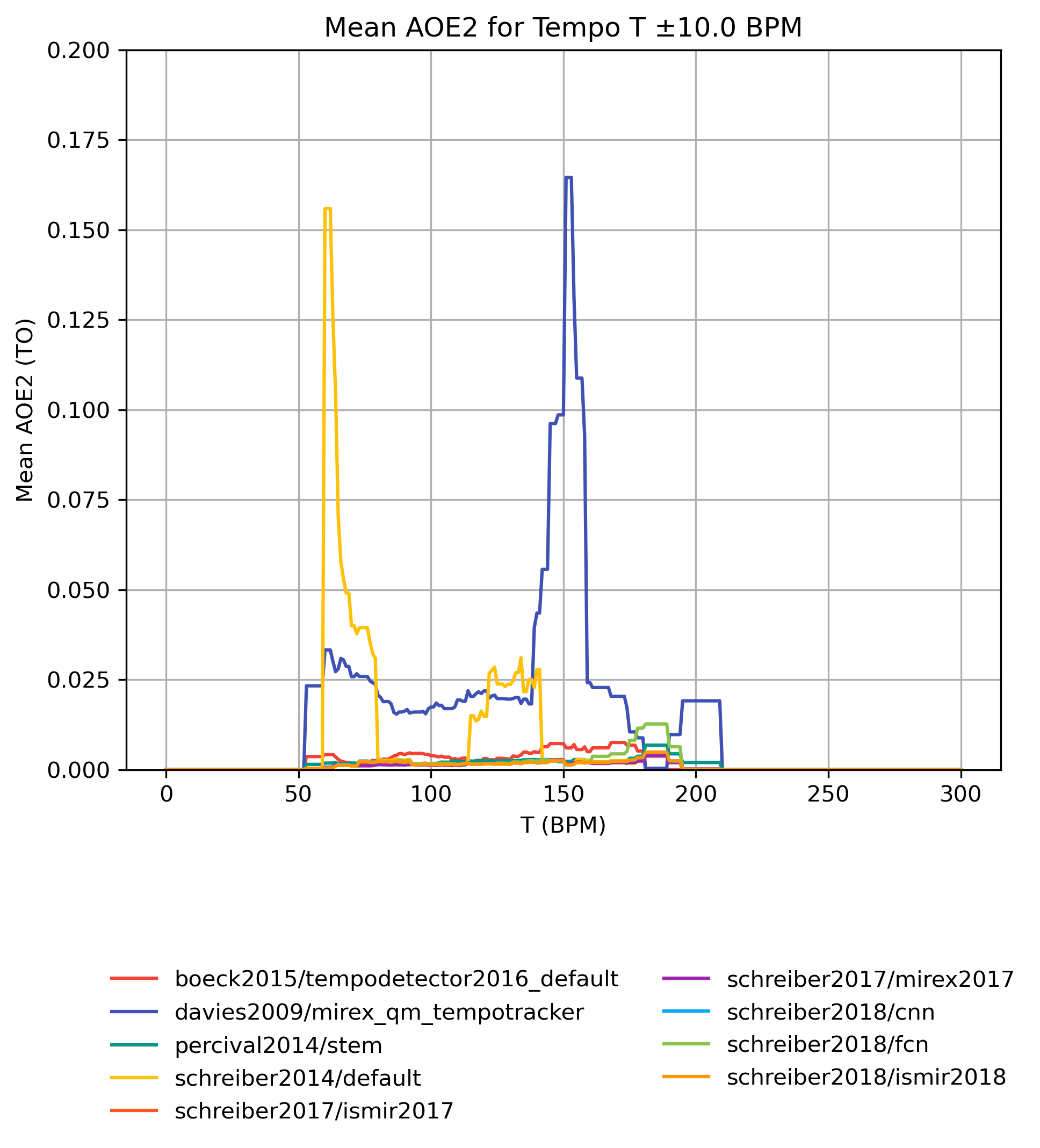
AOE2 on Tempo-Subsets for 1.0
Figure 56: Mean AOE2 for estimates compared to version 1.0 for tempo intervals around T.
CSV JSON LATEX PICKLE SVG PDF PNG
Estimated AOE1 for Tempo
When fitting a generalized additive model (GAM) to AOE1-values and a ground truth, what AOE1 can we expect with confidence?
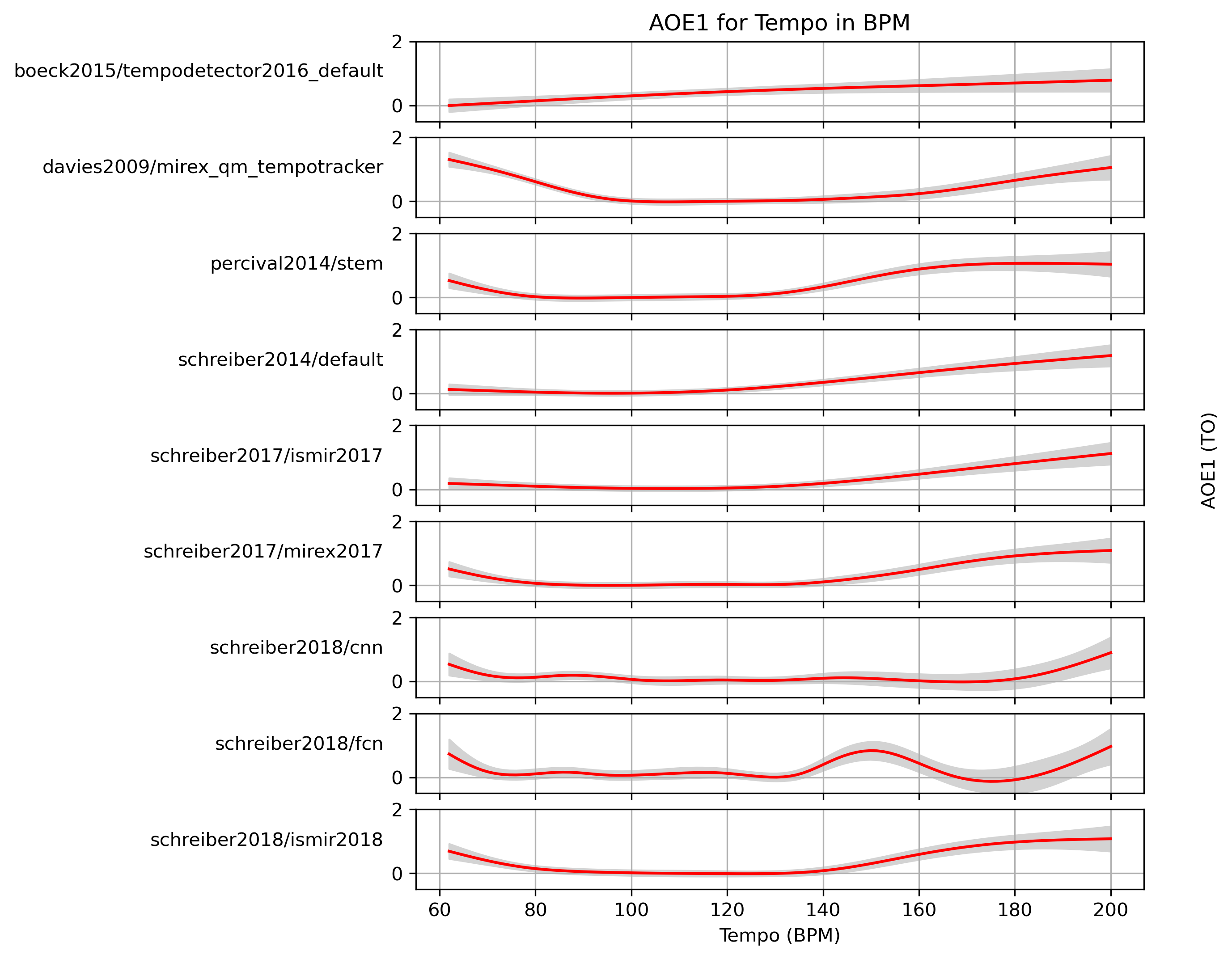
Estimated AOE1 for Tempo for 0.1
Predictions of GAMs trained on AOE1 for estimates for reference 0.1.
Figure 57: AOE1 predictions of a generalized additive model (GAM) fit to AOE1 results for 0.1. The 95% confidence interval around the prediction is shaded in gray.
CSV JSON LATEX PICKLE SVG PDF PNG
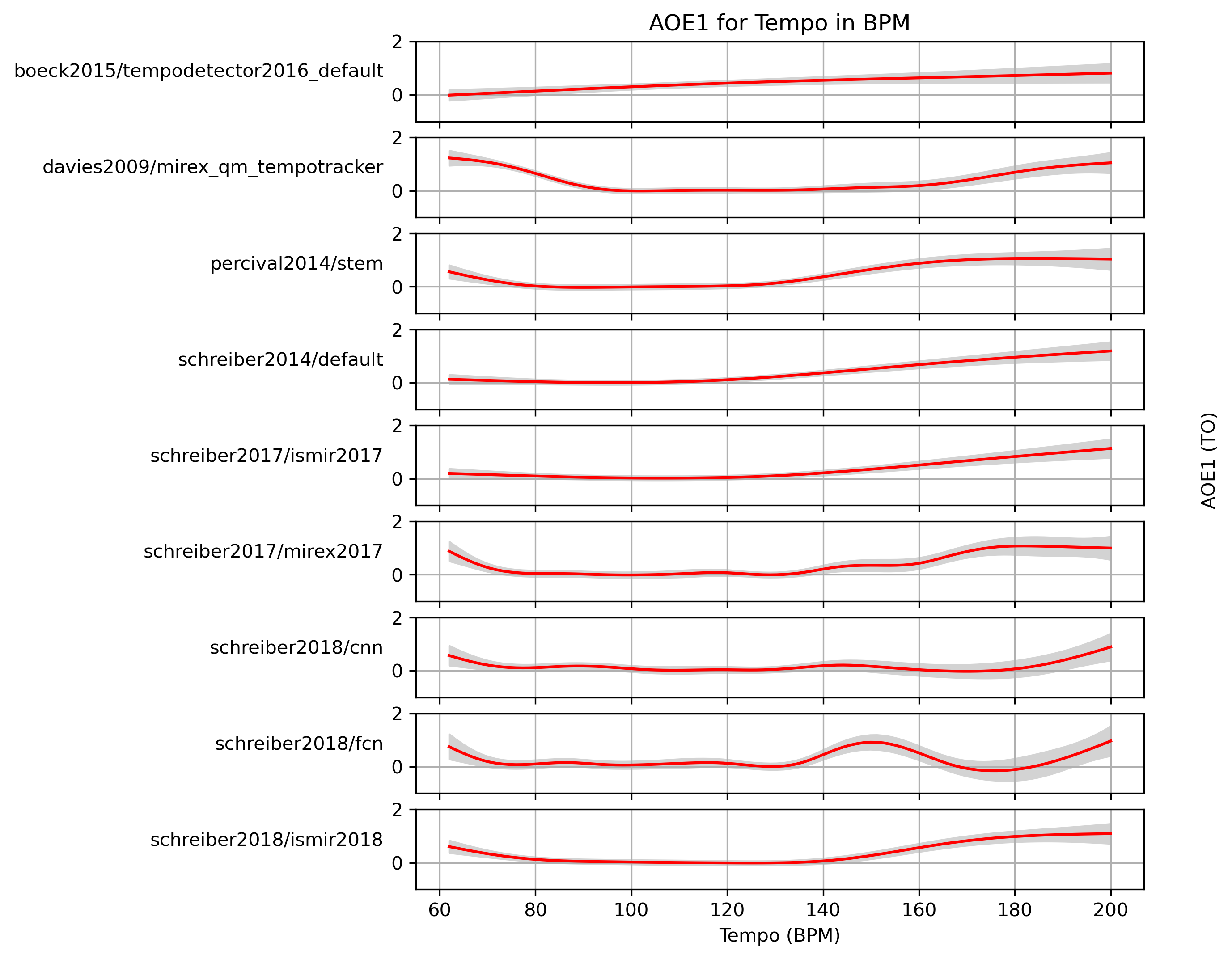
Estimated AOE1 for Tempo for 1.0
Predictions of GAMs trained on AOE1 for estimates for reference 1.0.
Figure 58: AOE1 predictions of a generalized additive model (GAM) fit to AOE1 results for 1.0. The 95% confidence interval around the prediction is shaded in gray.
CSV JSON LATEX PICKLE SVG PDF PNG
Estimated AOE2 for Tempo
When fitting a generalized additive model (GAM) to AOE2-values and a ground truth, what AOE2 can we expect with confidence?
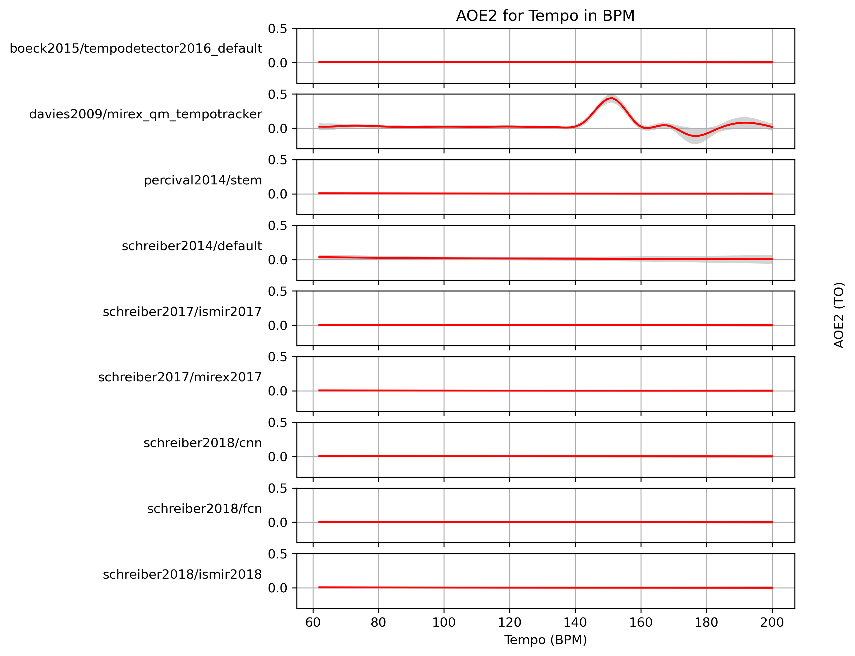
Estimated AOE2 for Tempo for 0.1
Predictions of GAMs trained on AOE2 for estimates for reference 0.1.
Figure 59: AOE2 predictions of a generalized additive model (GAM) fit to AOE2 results for 0.1. The 95% confidence interval around the prediction is shaded in gray.
CSV JSON LATEX PICKLE SVG PDF PNG
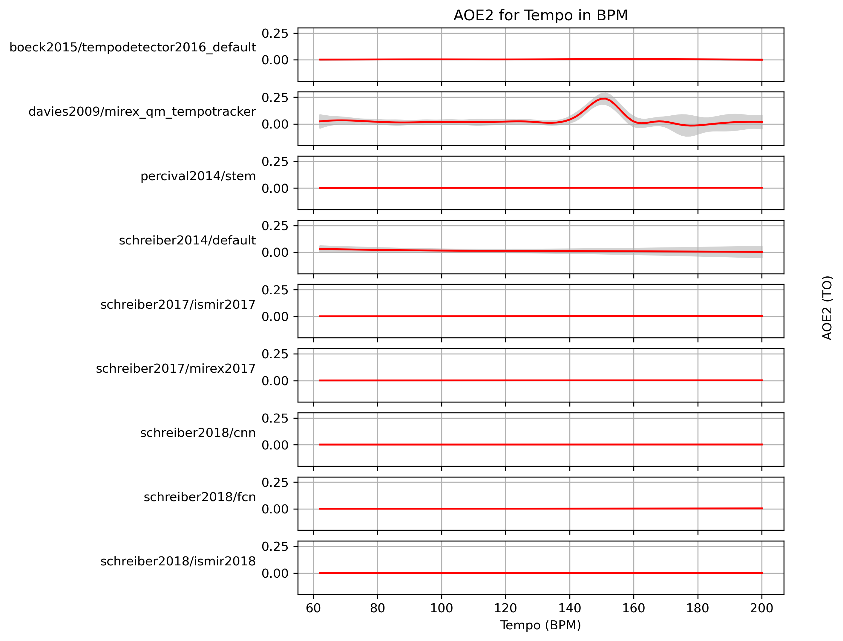
Estimated AOE2 for Tempo for 1.0
Predictions of GAMs trained on AOE2 for estimates for reference 1.0.
Figure 60: AOE2 predictions of a generalized additive model (GAM) fit to AOE2 results for 1.0. The 95% confidence interval around the prediction is shaded in gray.
CSV JSON LATEX PICKLE SVG PDF PNG
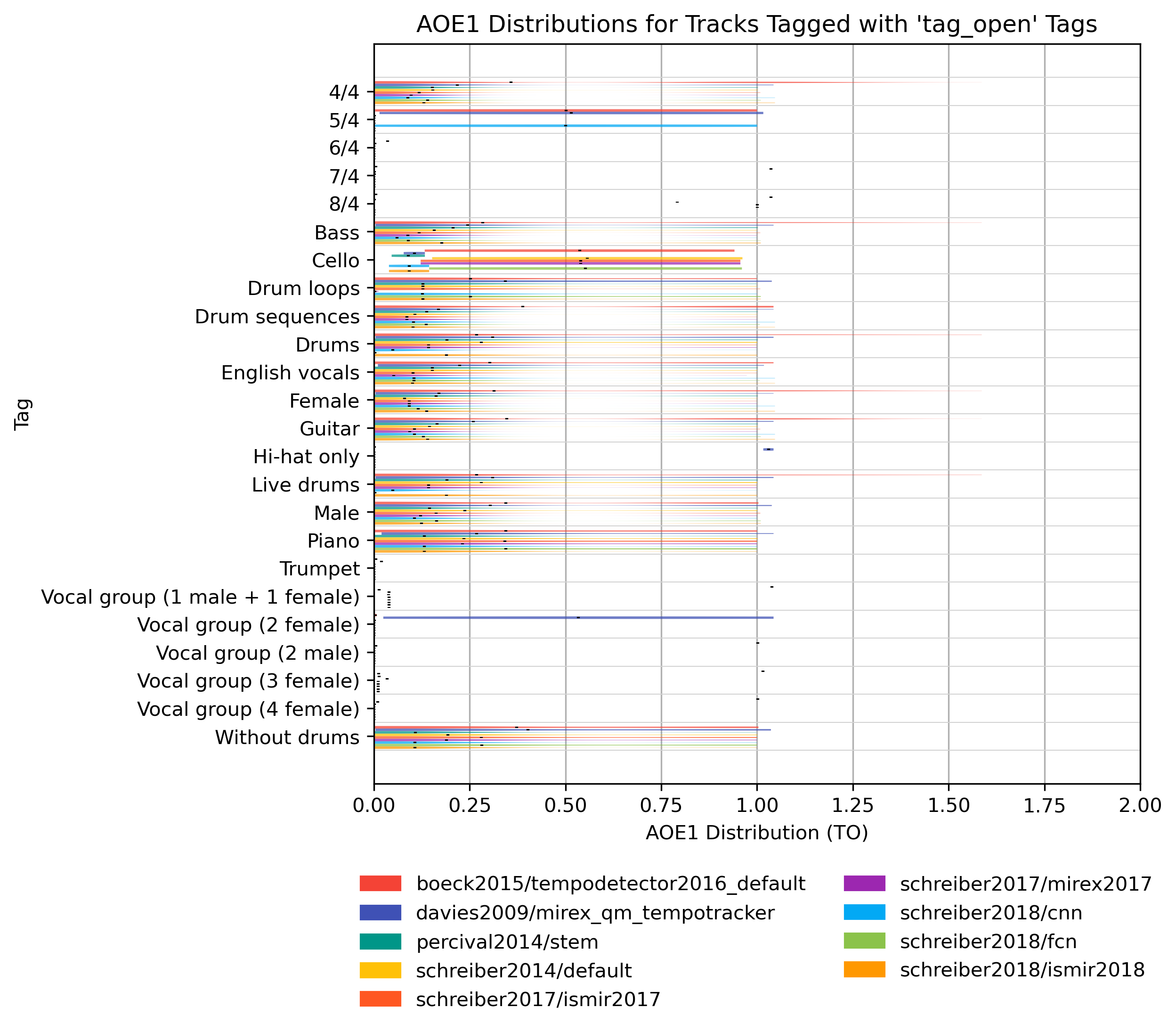
AOE1 for ‘tag_open’ Tags
How well does an estimator perform, when only taking tracks into account that are tagged with some kind of label? Note that some values may be based on very few estimates.
AOE1 for ‘tag_open’ Tags for 0.1
Figure 61: AOE1 of estimates compared to version 0.1 depending on tag from namespace ‘tag_open’.
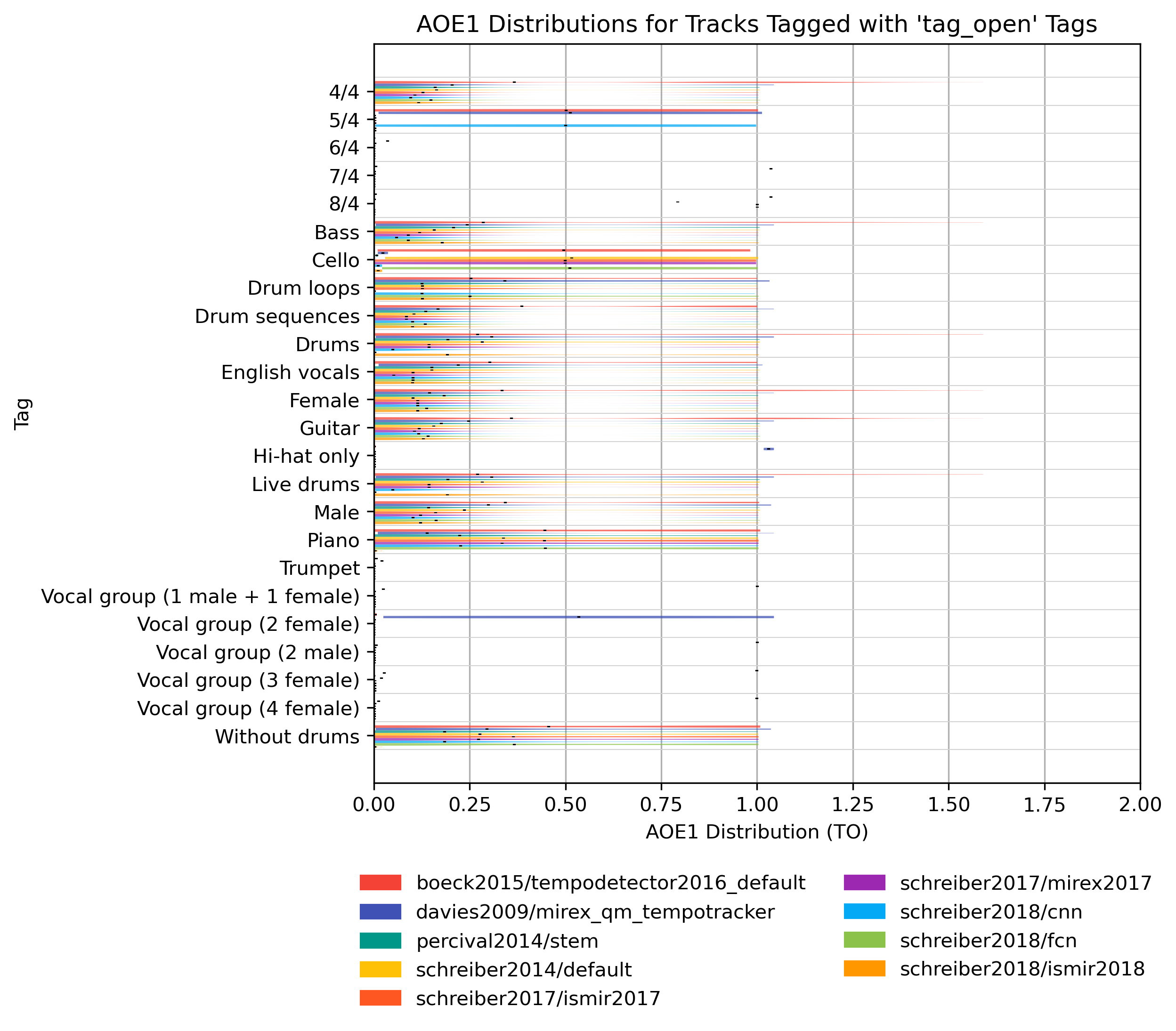
AOE1 for ‘tag_open’ Tags for 1.0
Figure 62: AOE1 of estimates compared to version 1.0 depending on tag from namespace ‘tag_open’.
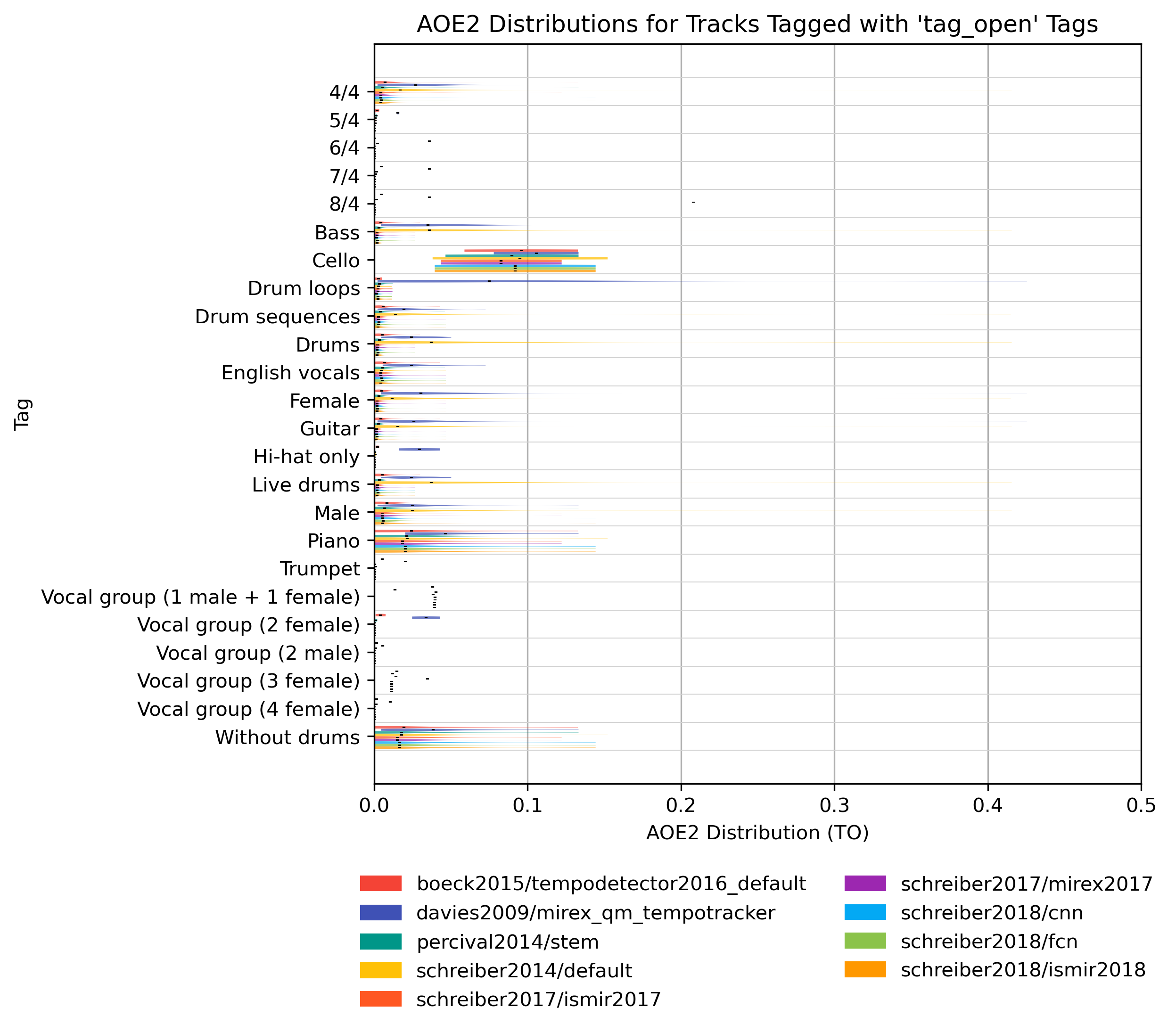
AOE2 for ‘tag_open’ Tags
How well does an estimator perform, when only taking tracks into account that are tagged with some kind of label? Note that some values may be based on very few estimates.
AOE2 for ‘tag_open’ Tags for 0.1
Figure 63: AOE2 of estimates compared to version 0.1 depending on tag from namespace ‘tag_open’.
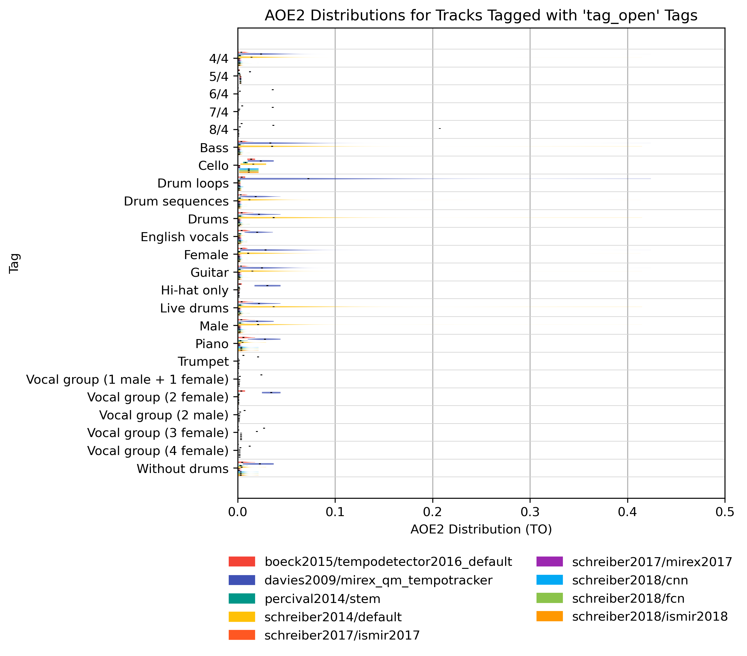
AOE2 for ‘tag_open’ Tags for 1.0
Figure 64: AOE2 of estimates compared to version 1.0 depending on tag from namespace ‘tag_open’.
Generated by tempo_eval 0.1.1 on 2022-06-29 18:54. Size L.