fma_medium
This is the tempo_eval report for the ‘fma_medium’ corpus.
Reports for other corpora may be found here.
Table of Contents
- References for ‘fma_medium’
- Estimates for ‘fma_medium’
- Estimators
- Basic Statistics
- Smoothed Tempo Distribution
- Accuracy
- Accuracy Results for schreiber2018/ismir2018
- Accuracy1 for schreiber2018/ismir2018
- Accuracy2 for schreiber2018/ismir2018
- Differing Items
- Significance of Differences
- Accuracy1 on Tempo-Subsets
- Accuracy2 on Tempo-Subsets
- Estimated Accuracy1 for Tempo
- Estimated Accuracy2 for Tempo
- Accuracy1 for ‘tag_fma_genre’ Tags
- Accuracy2 for ‘tag_fma_genre’ Tags
- MIREX-Style Evaluation
- MIREX Results for schreiber2018/ismir2018
- P-Score for schreiber2018/ismir2018
- One Correct for schreiber2018/ismir2018
- Both Correct for schreiber2018/ismir2018
- P-Score on Tempo-Subsets
- One Correct on Tempo-Subsets
- Both Correct on Tempo-Subsets
- Estimated P-Score for Tempo
- Estimated One Correct for Tempo
- Estimated Both Correct for Tempo
- P-Score for ‘tag_fma_genre’ Tags
- One Correct for ‘tag_fma_genre’ Tags
- Both Correct for ‘tag_fma_genre’ Tags
- OE1 and OE2
- Mean OE1/OE2 Results for schreiber2018/ismir2018
- OE1 distribution for schreiber2018/ismir2018
- OE2 distribution for schreiber2018/ismir2018
- Significance of Differences
- OE1 on Tempo-Subsets
- OE2 on Tempo-Subsets
- Estimated OE1 for Tempo
- Estimated OE2 for Tempo
- OE1 for ‘tag_fma_genre’ Tags
- OE2 for ‘tag_fma_genre’ Tags
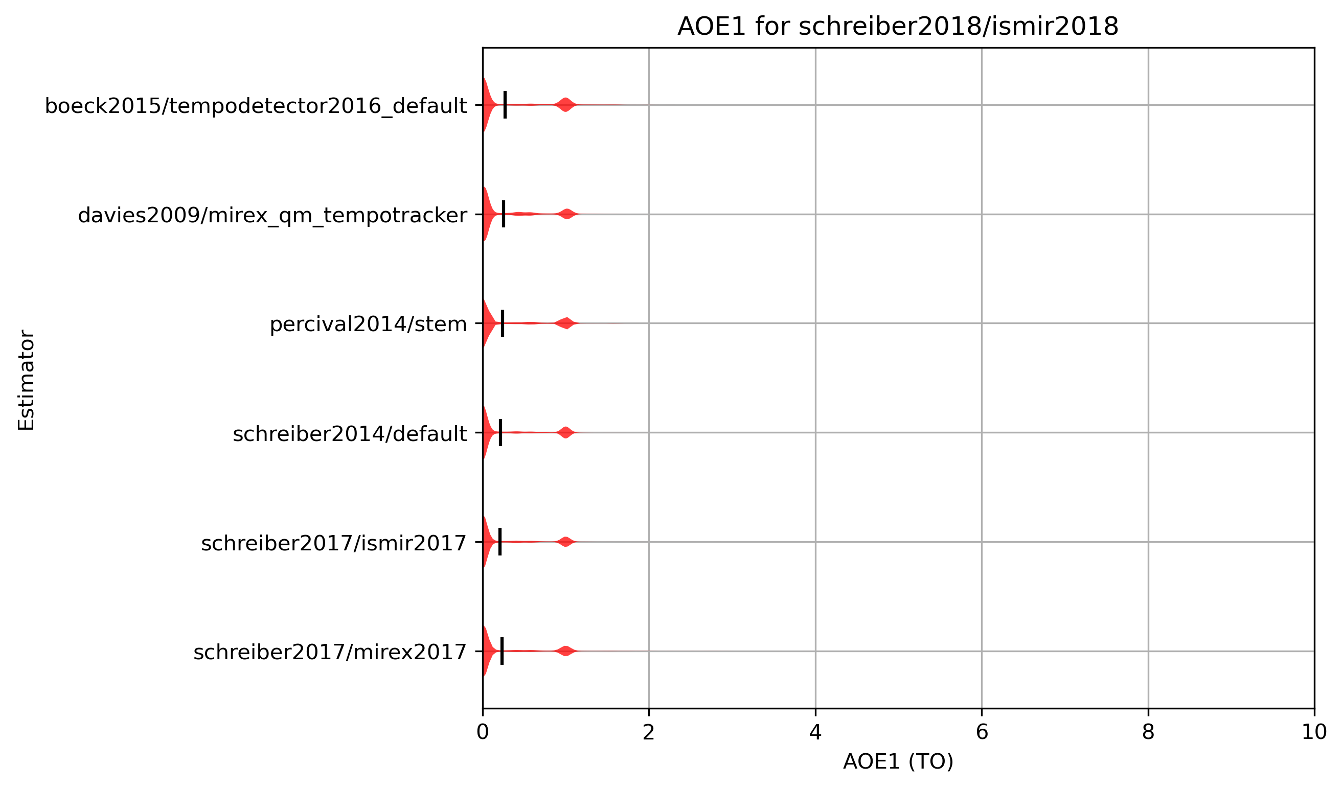
- AOE1 and AOE2
- Mean AOE1/AOE2 Results for schreiber2018/ismir2018
- AOE1 distribution for schreiber2018/ismir2018
- AOE2 distribution for schreiber2018/ismir2018
- Significance of Differences
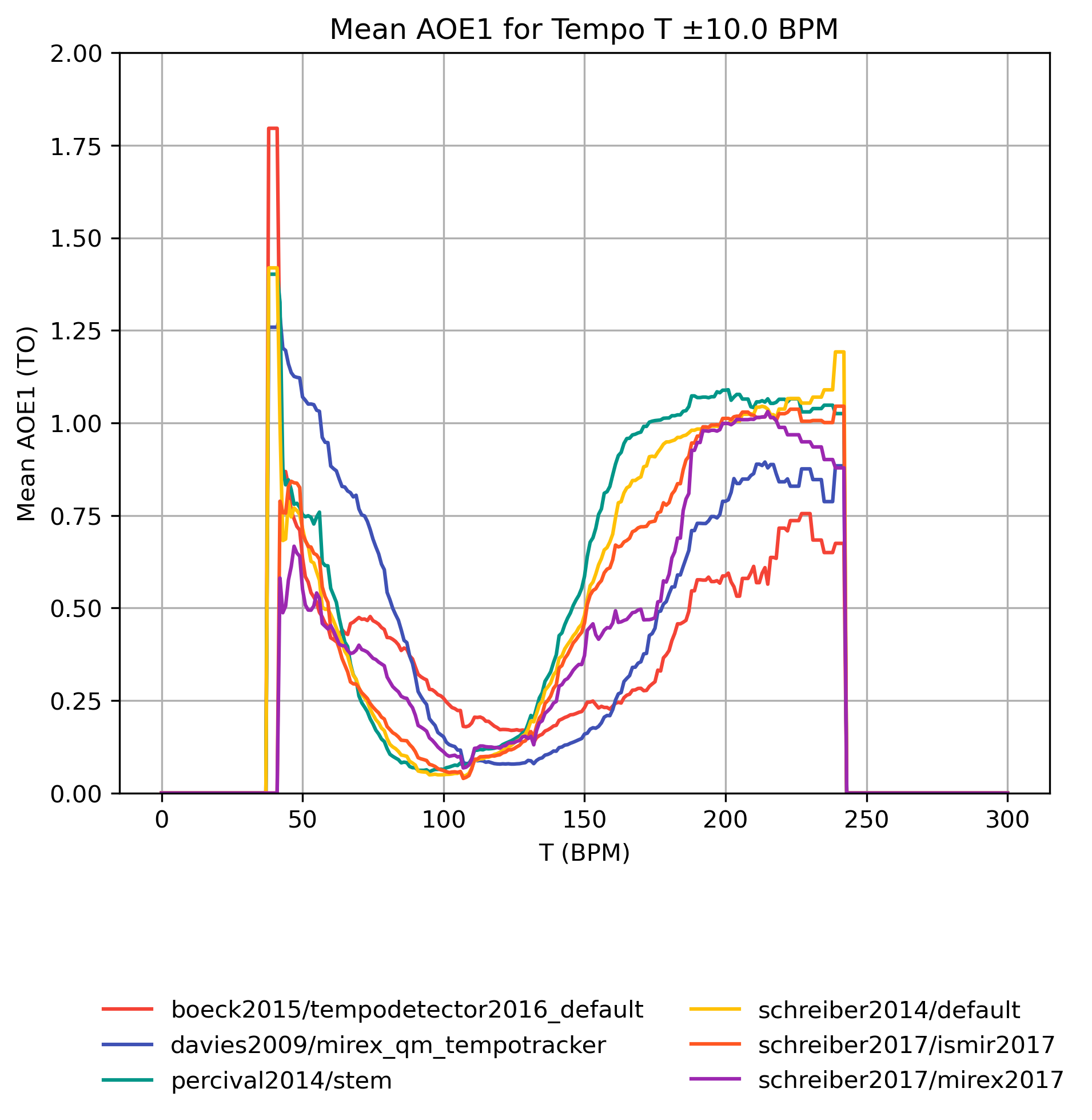
- AOE1 on Tempo-Subsets
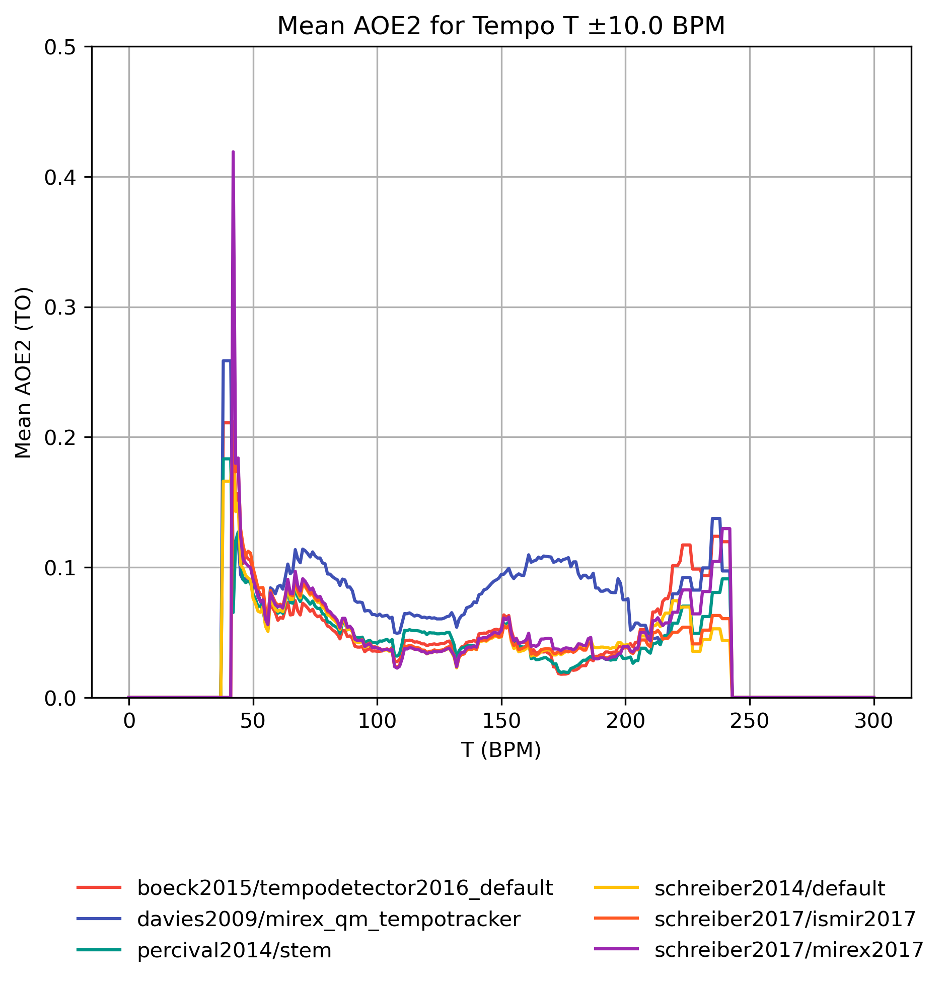
- AOE2 on Tempo-Subsets
- Estimated AOE1 for Tempo
- Estimated AOE2 for Tempo
- AOE1 for ‘tag_fma_genre’ Tags
- AOE2 for ‘tag_fma_genre’ Tags
Because reference annotations are not available, we treat the estimate schreiber2018/ismir2018 as reference. It has the highest Mean Mutual Agreement (MMA), based on Accuracy1 with 4% tolerance.
References for ‘fma_medium’
References
schreiber2018/ismir2018
| Attribute | Value |
|---|---|
| Corpus | |
| Version | 0.0.3 |
| Data Source | Hendrik Schreiber, Meinard Müller. A Single-Step Approach to Musical Tempo Estimation Using a Convolutional Neural Network. In Proceedings of the 19th International Society for Music Information Retrieval Conference (ISMIR), Paris, France, Sept. 2018. |
| Annotation Tools | schreiber tempo-cnn (model=ismir2018), https://github.com/hendriks73/tempo-cnn |
Basic Statistics
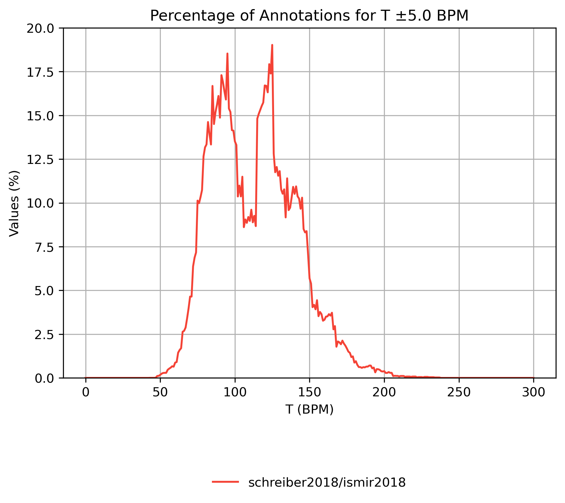
| Reference | Size | Min | Max | Avg | Stdev | Sweet Oct. Start | Sweet Oct. Coverage |
|---|---|---|---|---|---|---|---|
| schreiber2018/ismir2018 | 24983 | 48.00 | 232.00 | 113.24 | 27.62 | 77.00 | 0.87 |
Smoothed Tempo Distribution
Figure 1: Percentage of values in tempo interval.
CSV JSON LATEX PICKLE SVG PDF PNG
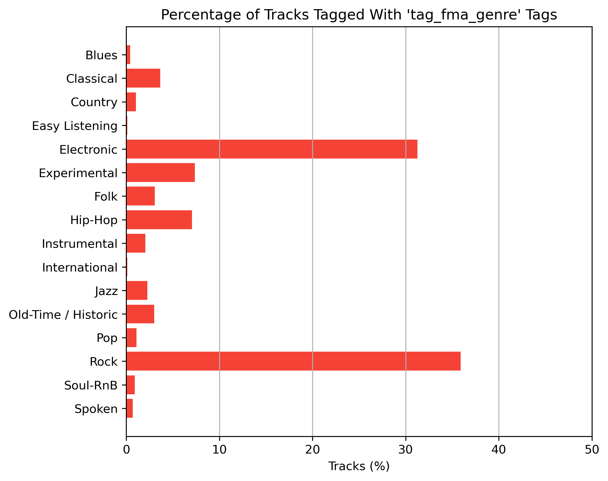
Tag Distribution for ‘tag_fma_genre’
Figure 2: Percentage of tracks tagged with tags from namespace ‘tag_fma_genre’. Annotations are from reference 1.0.0.
CSV JSON LATEX PICKLE SVG PDF PNG
Estimates for ‘fma_medium’
Estimators
boeck2015/tempodetector2016_default
| Attribute | Value |
|---|---|
| Corpus | fma_medium |
| Version | 0.17.dev0 |
| Annotation Tools | TempoDetector.2016, madmom, https://github.com/CPJKU/madmom |
| Annotator, bibtex | Boeck2015 |
davies2009/mirex_qm_tempotracker
| Attribute | Value | |
|---|---|---|
| Corpus | fma_medium | |
| Version | 1.0 | |
| Annotation Tools | QM Tempotracker, Sonic Annotator plugin. https://code.soundsoftware.ac.uk/projects/mirex2013/repository/show/audio_tempo_estimation/qm-tempotracker Note that the current macOS build of ‘qm-vamp-plugins’ was used. | |
| Annotator, bibtex | Davies2009 | Davies2007 |
percival2014/stem
| Attribute | Value |
|---|---|
| Corpus | fma_medium |
| Version | 1.0 |
| Annotation Tools | percival 2014, ‘tempo’ implementation from Marsyas, http://marsyas.info, git checkout tempo-stem |
| Annotator, bibtex | Percival2014 |
schreiber2014/default
| Attribute | Value |
|---|---|
| Corpus | fma_medium |
| Version | 0.0.1 |
| Annotation Tools | schreiber 2014, http://www.tagtraum.com/tempo_estimation.html |
| Annotator, bibtex | Schreiber2014 |
schreiber2017/ismir2017
| Attribute | Value |
|---|---|
| Corpus | fma_medium |
| Version | 0.0.4 |
| Annotation Tools | schreiber 2017, model=ismir2017, http://www.tagtraum.com/tempo_estimation.html |
| Annotator, bibtex | Schreiber2017 |
schreiber2017/mirex2017
| Attribute | Value |
|---|---|
| Corpus | fma_medium |
| Version | 0.0.4 |
| Annotation Tools | schreiber 2017, model=mirex2017, http://www.tagtraum.com/tempo_estimation.html |
| Annotator, bibtex | Schreiber2017 |
Basic Statistics
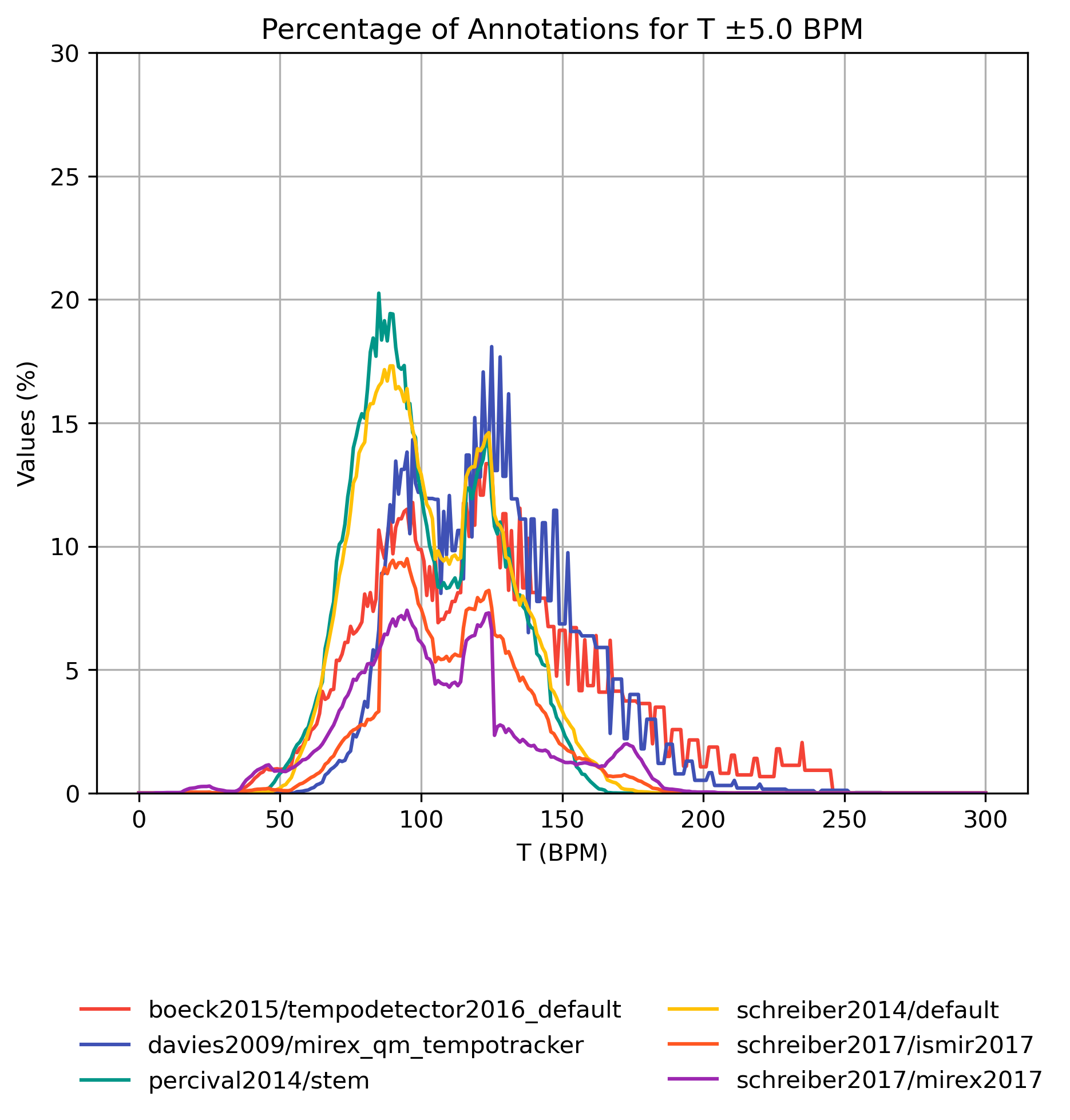
| Estimator | Size | Min | Max | Avg | Stdev | Sweet Oct. Start | Sweet Oct. Coverage |
|---|---|---|---|---|---|---|---|
| boeck2015/tempodetector2016_default | 24985 | 40.00 | 250.00 | 123.89 | 39.78 | 84.00 | 0.72 |
| davies2009/mirex_qm_tempotracker | 24946 | 58.07 | 258.40 | 125.08 | 28.83 | 87.00 | 0.88 |
| percival2014/stem | 24985 | 50.17 | inf | inf | nan | 72.00 | 0.88 |
| schreiber2014/default | 24951 | 40.18 | 182.00 | 104.04 | 24.07 | 72.00 | 0.87 |
| schreiber2017/ismir2017 | 24982 | 15.85 | 208.10 | 105.09 | 26.18 | 72.00 | 0.85 |
| schreiber2017/mirex2017 | 24982 | 10.01 | 216.07 | 108.16 | 30.57 | 75.00 | 0.78 |
Smoothed Tempo Distribution
Figure 3: Percentage of values in tempo interval.
CSV JSON LATEX PICKLE SVG PDF PNG
Accuracy
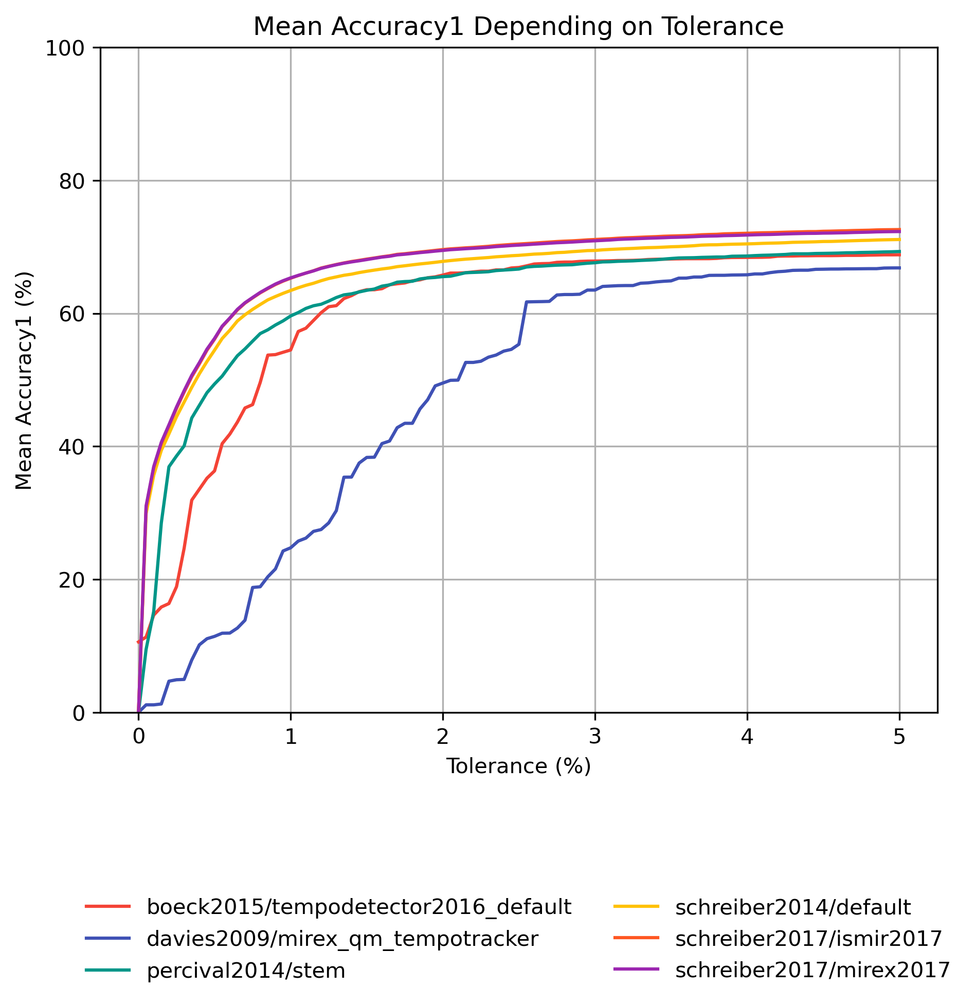
Accuracy1 is defined as the percentage of correct estimates, allowing a 4% tolerance for individual BPM values.
Accuracy2 additionally permits estimates to be wrong by a factor of 2, 3, 1/2 or 1/3 (so-called octave errors).
See [Gouyon2006].
Note: When comparing accuracy values for different algorithms, keep in mind that an algorithm may have been trained on the test set or that the test set may have even been created using one of the tested algorithms.
Accuracy Results for schreiber2018/ismir2018
| Estimator | Accuracy1 | Accuracy2 |
|---|---|---|
| schreiber2017/ismir2017 | 0.7205 | 0.8595 |
| schreiber2017/mirex2017 | 0.7178 | 0.8612 |
| schreiber2014/default | 0.7045 | 0.8601 |
| percival2014/stem | 0.6863 | 0.8536 |
| boeck2015/tempodetector2016_default | 0.6841 | 0.8713 |
| davies2009/mirex_qm_tempotracker | 0.6580 | 0.7945 |
Table 3: Mean accuracy of estimates compared to version schreiber2018/ismir2018 with 4% tolerance ordered by Accuracy1.
Raw data Accuracy1: CSV JSON LATEX PICKLE
Raw data Accuracy2: CSV JSON LATEX PICKLE
Accuracy1 for schreiber2018/ismir2018
Figure 4: Mean Accuracy1 for estimates compared to version schreiber2018/ismir2018 depending on tolerance.
CSV JSON LATEX PICKLE SVG PDF PNG
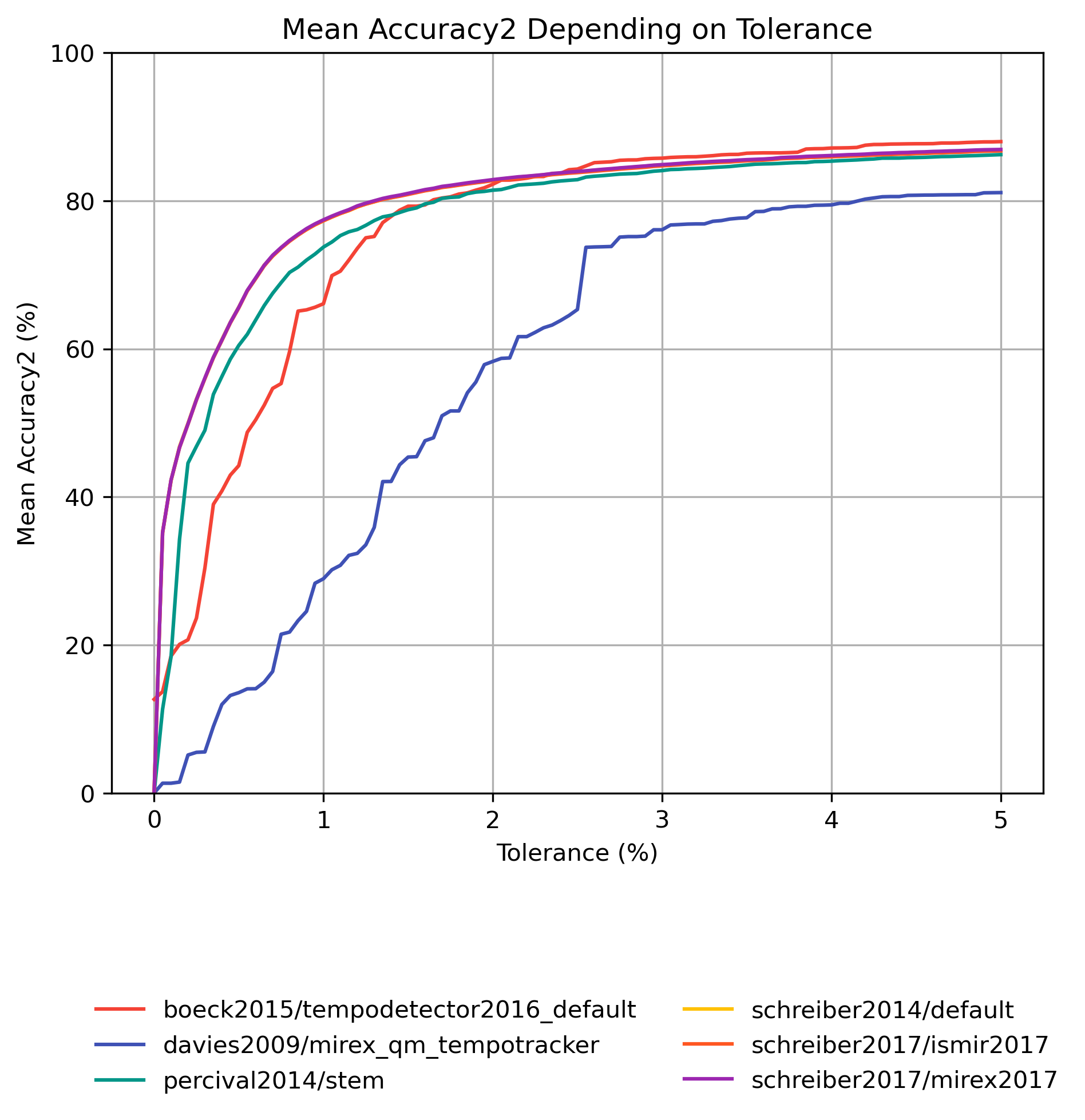
Accuracy2 for schreiber2018/ismir2018
Figure 5: Mean Accuracy2 for estimates compared to version schreiber2018/ismir2018 depending on tolerance.
CSV JSON LATEX PICKLE SVG PDF PNG
Differing Items
For which items did a given estimator not estimate a correct value with respect to a given ground truth? Are there items which are either very difficult, not suitable for the task, or incorrectly annotated and therefore never estimated correctly, regardless which estimator is used?
Differing Items Accuracy1
Items with different tempo annotations (Accuracy1, 4% tolerance) in different versions:
schreiber2018/ismir2018 compared with boeck2015/tempodetector2016_default (7891 differences): ‘000/000003’ ‘000/000140’ ‘000/000148’ ‘000/000181’ ‘000/000193’ ‘000/000197’ ‘000/000200’ ‘000/000207’ ‘000/000208’ ‘000/000210’ ‘000/000249’ … CSV
schreiber2018/ismir2018 compared with davies2009/mirex_qm_tempotracker (8544 differences): ‘000/000003’ ‘000/000148’ ‘000/000181’ ‘000/000194’ ‘000/000197’ ‘000/000200’ ‘000/000207’ ‘000/000210’ ‘000/000249’ ‘000/000256’ ‘000/000258’ … CSV
schreiber2018/ismir2018 compared with percival2014/stem (7838 differences): ‘000/000141’ ‘000/000148’ ‘000/000181’ ‘000/000193’ ‘000/000194’ ‘000/000197’ ‘000/000200’ ‘000/000237’ ‘000/000256’ ‘000/000341’ ‘000/000343’ … CSV
schreiber2018/ismir2018 compared with schreiber2014/default (7383 differences): ‘000/000140’ ‘000/000148’ ‘000/000181’ ‘000/000182’ ‘000/000194’ ‘000/000197’ ‘000/000200’ ‘000/000258’ ‘000/000343’ ‘000/000397’ ‘000/000399’ … CSV
schreiber2018/ismir2018 compared with schreiber2017/ismir2017 (6983 differences): ‘000/000136’ ‘000/000141’ ‘000/000148’ ‘000/000181’ ‘000/000194’ ‘000/000207’ ‘000/000247’ ‘000/000258’ ‘000/000341’ ‘000/000343’ ‘000/000397’ … CSV
schreiber2018/ismir2018 compared with schreiber2017/mirex2017 (7050 differences): ‘000/000136’ ‘000/000141’ ‘000/000148’ ‘000/000181’ ‘000/000182’ ‘000/000194’ ‘000/000197’ ‘000/000207’ ‘000/000247’ ‘000/000258’ ‘000/000341’ … CSV
None of the estimators estimated the following 2257 items ‘correctly’ using Accuracy1: ‘000/000148’ ‘000/000181’ ‘000/000399’ ‘000/000400’ ‘000/000405’ ‘000/000414’ ‘000/000540’ ‘000/000676’ ‘000/000677’ ‘000/000714’ ‘000/000715’ … CSV
Differing Items Accuracy2
Items with different tempo annotations (Accuracy2, 4% tolerance) in different versions:
schreiber2018/ismir2018 compared with boeck2015/tempodetector2016_default (3215 differences): ‘000/000140’ ‘000/000148’ ‘000/000197’ ‘000/000207’ ‘000/000258’ ‘000/000399’ ‘000/000405’ ‘000/000414’ ‘000/000424’ ‘000/000425’ ‘000/000535’ … CSV
schreiber2018/ismir2018 compared with davies2009/mirex_qm_tempotracker (5134 differences): ‘000/000003’ ‘000/000148’ ‘000/000194’ ‘000/000197’ ‘000/000200’ ‘000/000210’ ‘000/000249’ ‘000/000256’ ‘000/000258’ ‘000/000343’ ‘000/000397’ … CSV
schreiber2018/ismir2018 compared with percival2014/stem (3658 differences): ‘000/000141’ ‘000/000148’ ‘000/000194’ ‘000/000197’ ‘000/000200’ ‘000/000341’ ‘000/000343’ ‘000/000397’ ‘000/000399’ ‘000/000400’ ‘000/000405’ … CSV
schreiber2018/ismir2018 compared with schreiber2014/default (3495 differences): ‘000/000140’ ‘000/000148’ ‘000/000181’ ‘000/000194’ ‘000/000197’ ‘000/000200’ ‘000/000258’ ‘000/000397’ ‘000/000399’ ‘000/000400’ ‘000/000405’ … CSV
schreiber2018/ismir2018 compared with schreiber2017/ismir2017 (3509 differences): ‘000/000141’ ‘000/000148’ ‘000/000181’ ‘000/000194’ ‘000/000258’ ‘000/000341’ ‘000/000397’ ‘000/000399’ ‘000/000400’ ‘000/000405’ ‘000/000414’ … CSV
schreiber2018/ismir2018 compared with schreiber2017/mirex2017 (3467 differences): ‘000/000141’ ‘000/000148’ ‘000/000181’ ‘000/000194’ ‘000/000258’ ‘000/000341’ ‘000/000397’ ‘000/000399’ ‘000/000400’ ‘000/000405’ ‘000/000424’ … CSV
None of the estimators estimated the following 1415 items ‘correctly’ using Accuracy2: ‘000/000148’ ‘000/000399’ ‘000/000405’ ‘000/000540’ ‘000/000714’ ‘000/000715’ ‘000/000753’ ‘000/000819’ ‘000/000878’ ‘000/000890’ ‘000/000995’ … CSV
Significance of Differences
| Estimator | boeck2015/tempodetector2016_default | davies2009/mirex_qm_tempotracker | percival2014/stem | schreiber2014/default | schreiber2017/ismir2017 | schreiber2017/mirex2017 |
|---|---|---|---|---|---|---|
| boeck2015/tempodetector2016_default | 1.0000 | 0.0000 | 0.5337 | 0.0000 | 0.0000 | 0.0000 |
| davies2009/mirex_qm_tempotracker | 0.0000 | 1.0000 | 0.0000 | 0.0000 | 0.0000 | 0.0000 |
| percival2014/stem | 0.5337 | 0.0000 | 1.0000 | 0.0000 | 0.0000 | 0.0000 |
| schreiber2014/default | 0.0000 | 0.0000 | 0.0000 | 1.0000 | 0.0000 | 0.0000 |
| schreiber2017/ismir2017 | 0.0000 | 0.0000 | 0.0000 | 0.0000 | 1.0000 | 0.1700 |
| schreiber2017/mirex2017 | 0.0000 | 0.0000 | 0.0000 | 0.0000 | 0.1700 | 1.0000 |
Table 4: McNemar p-values, using reference annotations schreiber2018/ismir2018 as groundtruth with Accuracy1 [Gouyon2006]. H0: both estimators disagree with the groundtruth to the same amount. If p<=ɑ, reject H0, i.e. we have a significant difference in the disagreement with the groundtruth. In the table, p-values<0.05 are set in bold.
| Estimator | boeck2015/tempodetector2016_default | davies2009/mirex_qm_tempotracker | percival2014/stem | schreiber2014/default | schreiber2017/ismir2017 | schreiber2017/mirex2017 |
|---|---|---|---|---|---|---|
| boeck2015/tempodetector2016_default | 1.0000 | 0.0000 | 0.0000 | 0.0000 | 0.0000 | 0.0000 |
| davies2009/mirex_qm_tempotracker | 0.0000 | 1.0000 | 0.0000 | 0.0000 | 0.0000 | 0.0000 |
| percival2014/stem | 0.0000 | 0.0000 | 1.0000 | 0.0014 | 0.0037 | 0.0002 |
| schreiber2014/default | 0.0000 | 0.0000 | 0.0014 | 1.0000 | 0.6987 | 0.4247 |
| schreiber2017/ismir2017 | 0.0000 | 0.0000 | 0.0037 | 0.6987 | 1.0000 | 0.0021 |
| schreiber2017/mirex2017 | 0.0000 | 0.0000 | 0.0002 | 0.4247 | 0.0021 | 1.0000 |
Table 5: McNemar p-values, using reference annotations schreiber2018/ismir2018 as groundtruth with Accuracy2 [Gouyon2006]. H0: both estimators disagree with the groundtruth to the same amount. If p<=ɑ, reject H0, i.e. we have a significant difference in the disagreement with the groundtruth. In the table, p-values<0.05 are set in bold.
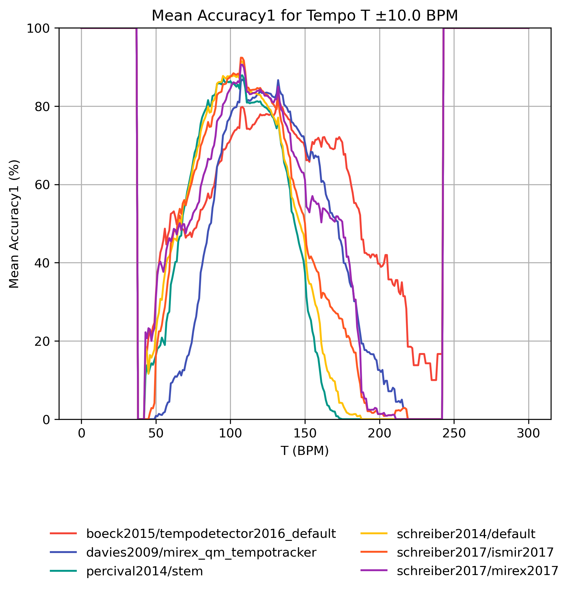
Accuracy1 on Tempo-Subsets
How well does an estimator perform, when only taking a subset of the reference annotations into account? The graphs show mean Accuracy1 for reference subsets with tempi in [T-10,T+10] BPM. Note that the graphs do not show confidence intervals and that some values may be based on very few estimates.
Accuracy1 on Tempo-Subsets for schreiber2018/ismir2018
Figure 6: Mean Accuracy1 for estimates compared to version schreiber2018/ismir2018 for tempo intervals around T.
CSV JSON LATEX PICKLE SVG PDF PNG
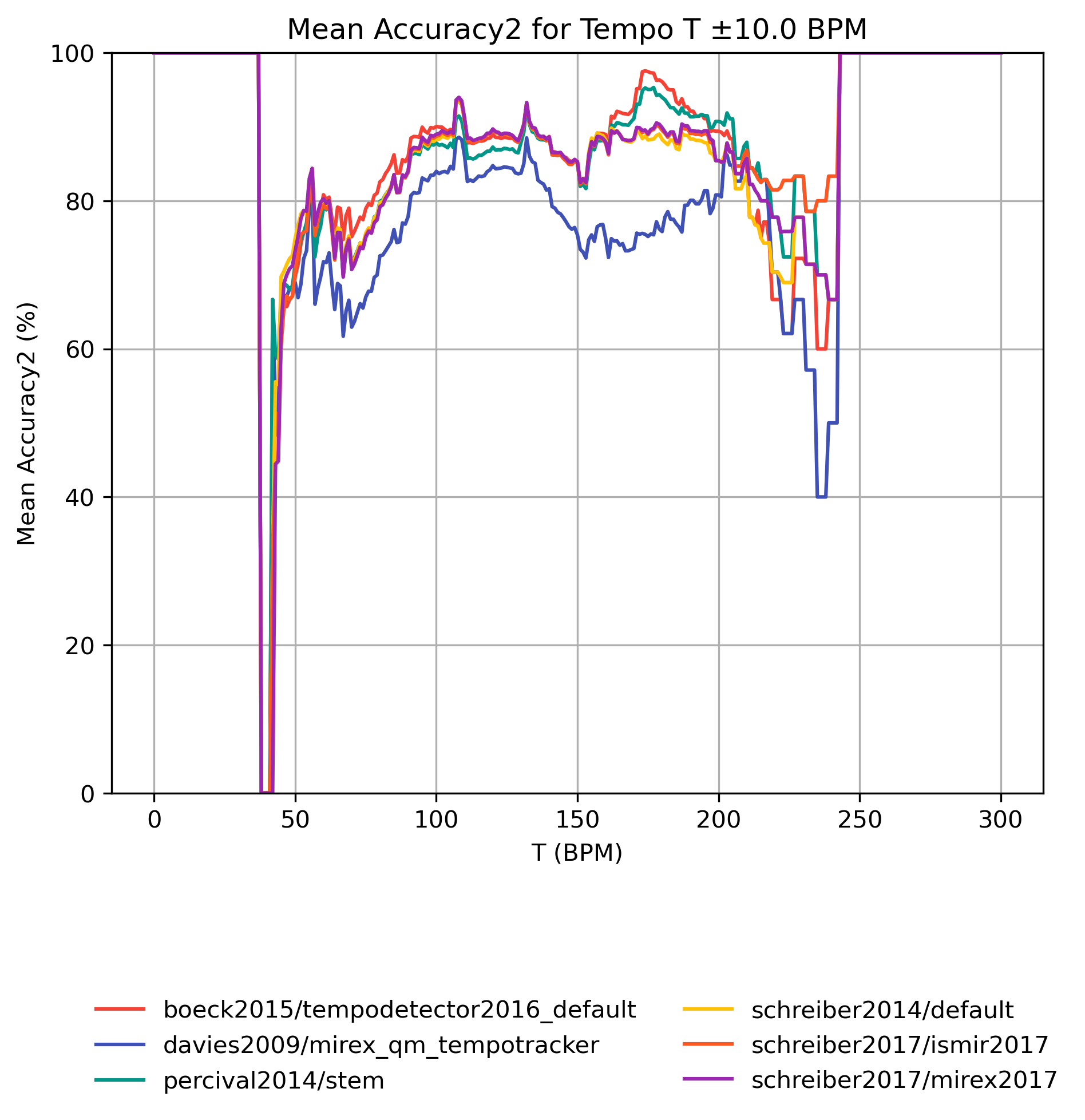
Accuracy2 on Tempo-Subsets
How well does an estimator perform, when only taking a subset of the reference annotations into account? The graphs show mean Accuracy2 for reference subsets with tempi in [T-10,T+10] BPM. Note that the graphs do not show confidence intervals and that some values may be based on very few estimates.
Accuracy2 on Tempo-Subsets for schreiber2018/ismir2018
Figure 7: Mean Accuracy2 for estimates compared to version schreiber2018/ismir2018 for tempo intervals around T.
CSV JSON LATEX PICKLE SVG PDF PNG
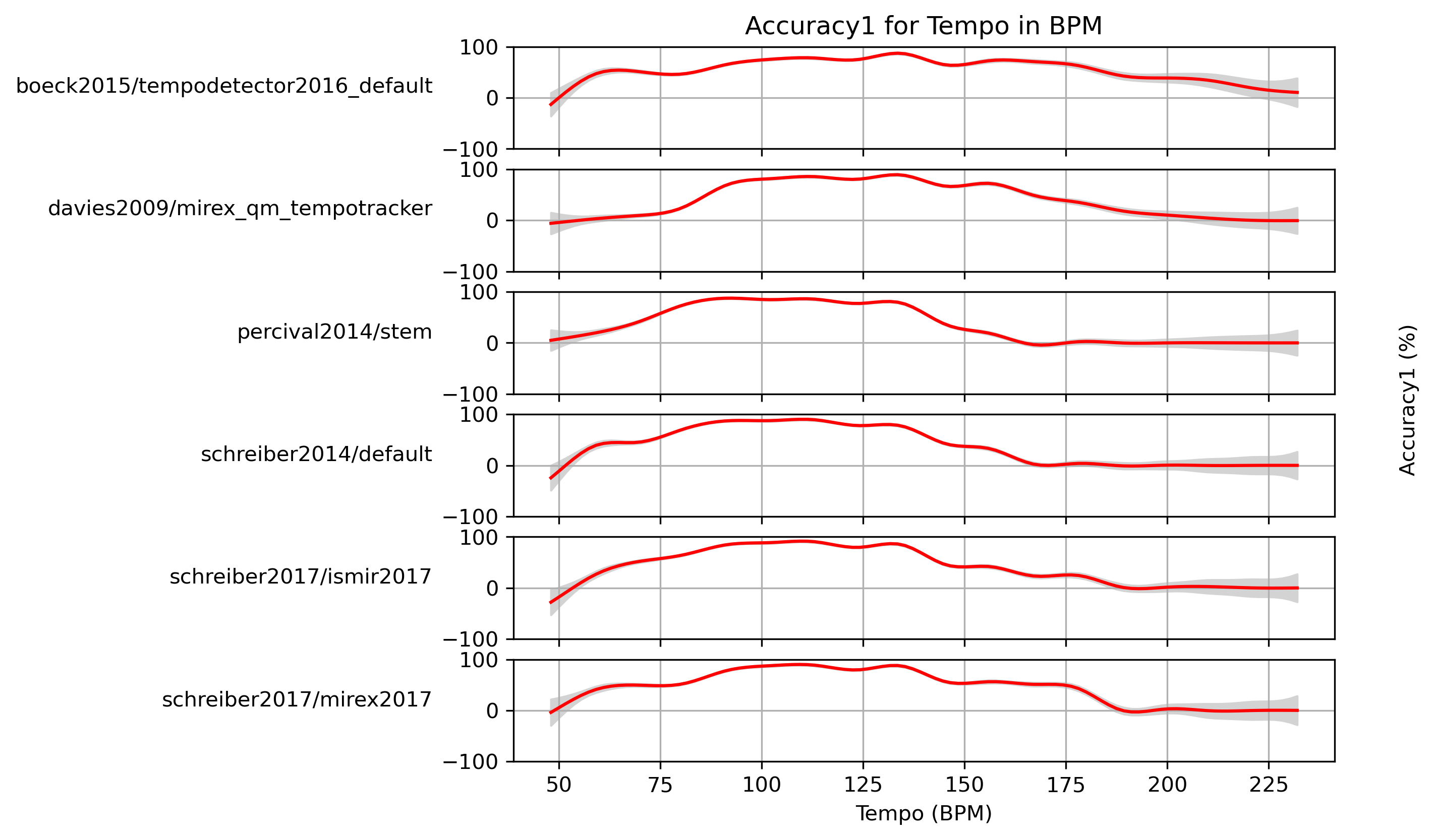
Estimated Accuracy1 for Tempo
When fitting a generalized additive model (GAM) to Accuracy1-values and a ground truth, what Accuracy1 can we expect with confidence?
Estimated Accuracy1 for Tempo for schreiber2018/ismir2018
Predictions of GAMs trained on Accuracy1 for estimates for reference schreiber2018/ismir2018.
Figure 8: Accuracy1 predictions of a generalized additive model (GAM) fit to Accuracy1 results for schreiber2018/ismir2018. The 95% confidence interval around the prediction is shaded in gray.
CSV JSON LATEX PICKLE SVG PDF PNG
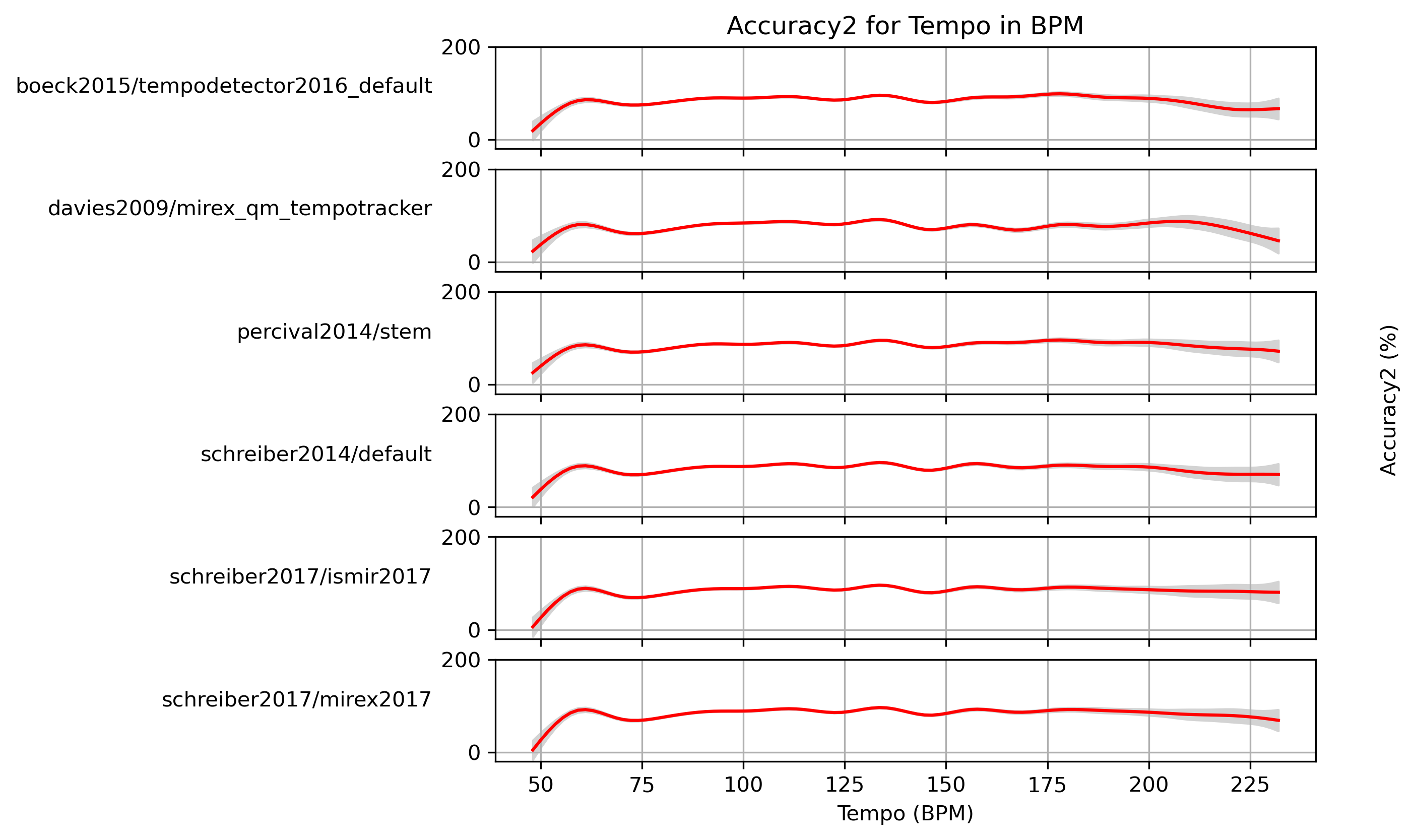
Estimated Accuracy2 for Tempo
When fitting a generalized additive model (GAM) to Accuracy2-values and a ground truth, what Accuracy2 can we expect with confidence?
Estimated Accuracy2 for Tempo for schreiber2018/ismir2018
Predictions of GAMs trained on Accuracy2 for estimates for reference schreiber2018/ismir2018.
Figure 9: Accuracy2 predictions of a generalized additive model (GAM) fit to Accuracy2 results for schreiber2018/ismir2018. The 95% confidence interval around the prediction is shaded in gray.
CSV JSON LATEX PICKLE SVG PDF PNG
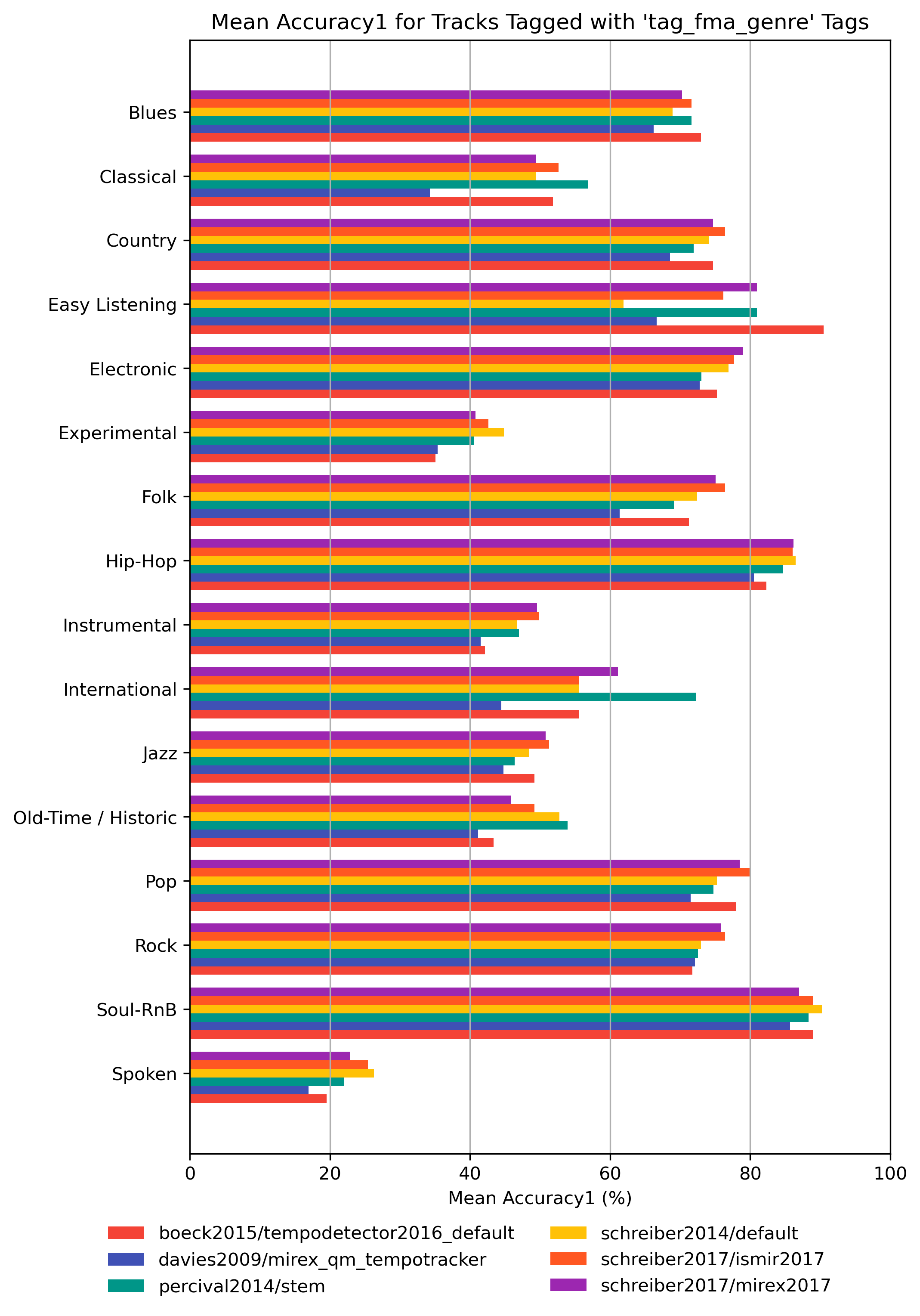
Accuracy1 for ‘tag_fma_genre’ Tags
How well does an estimator perform, when only taking tracks into account that are tagged with some kind of label? Note that some values may be based on very few estimates.
Accuracy1 for ‘tag_fma_genre’ Tags for schreiber2018/ismir2018
Figure 10: Mean Accuracy1 of estimates compared to version schreiber2018/ismir2018 depending on tag from namespace ‘tag_fma_genre’.
CSV JSON LATEX PICKLE SVG PDF PNG
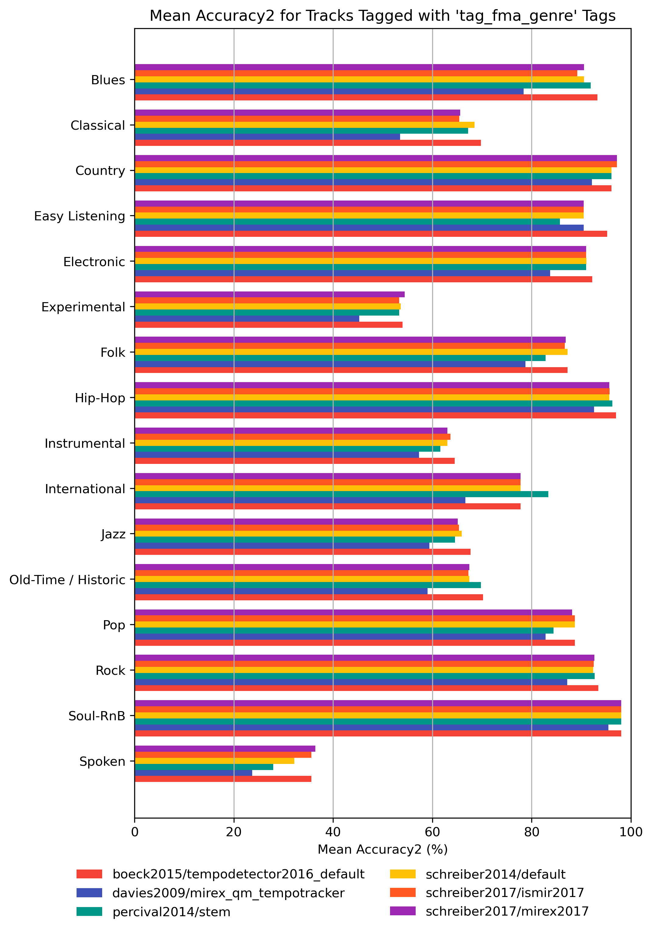
Accuracy2 for ‘tag_fma_genre’ Tags
How well does an estimator perform, when only taking tracks into account that are tagged with some kind of label? Note that some values may be based on very few estimates.
Accuracy2 for ‘tag_fma_genre’ Tags for schreiber2018/ismir2018
Figure 11: Mean Accuracy2 of estimates compared to version schreiber2018/ismir2018 depending on tag from namespace ‘tag_fma_genre’.
CSV JSON LATEX PICKLE SVG PDF PNG
MIREX-Style Evaluation
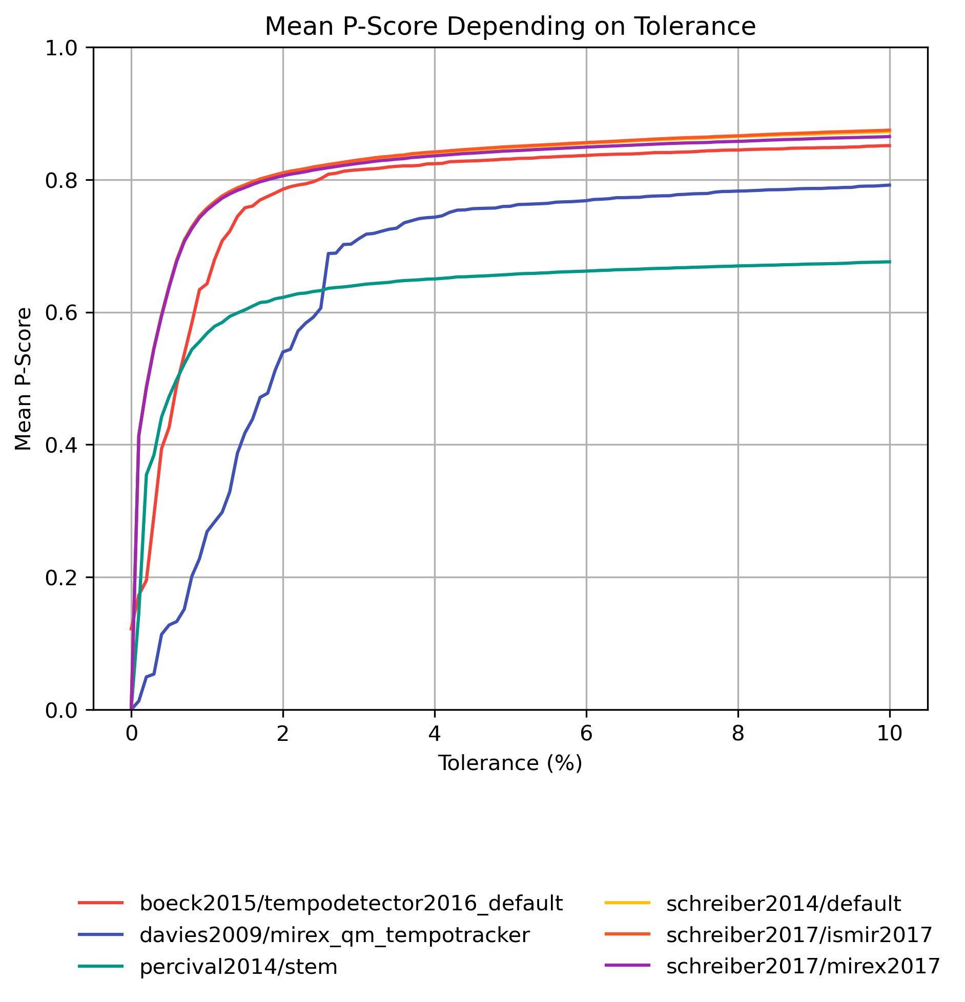
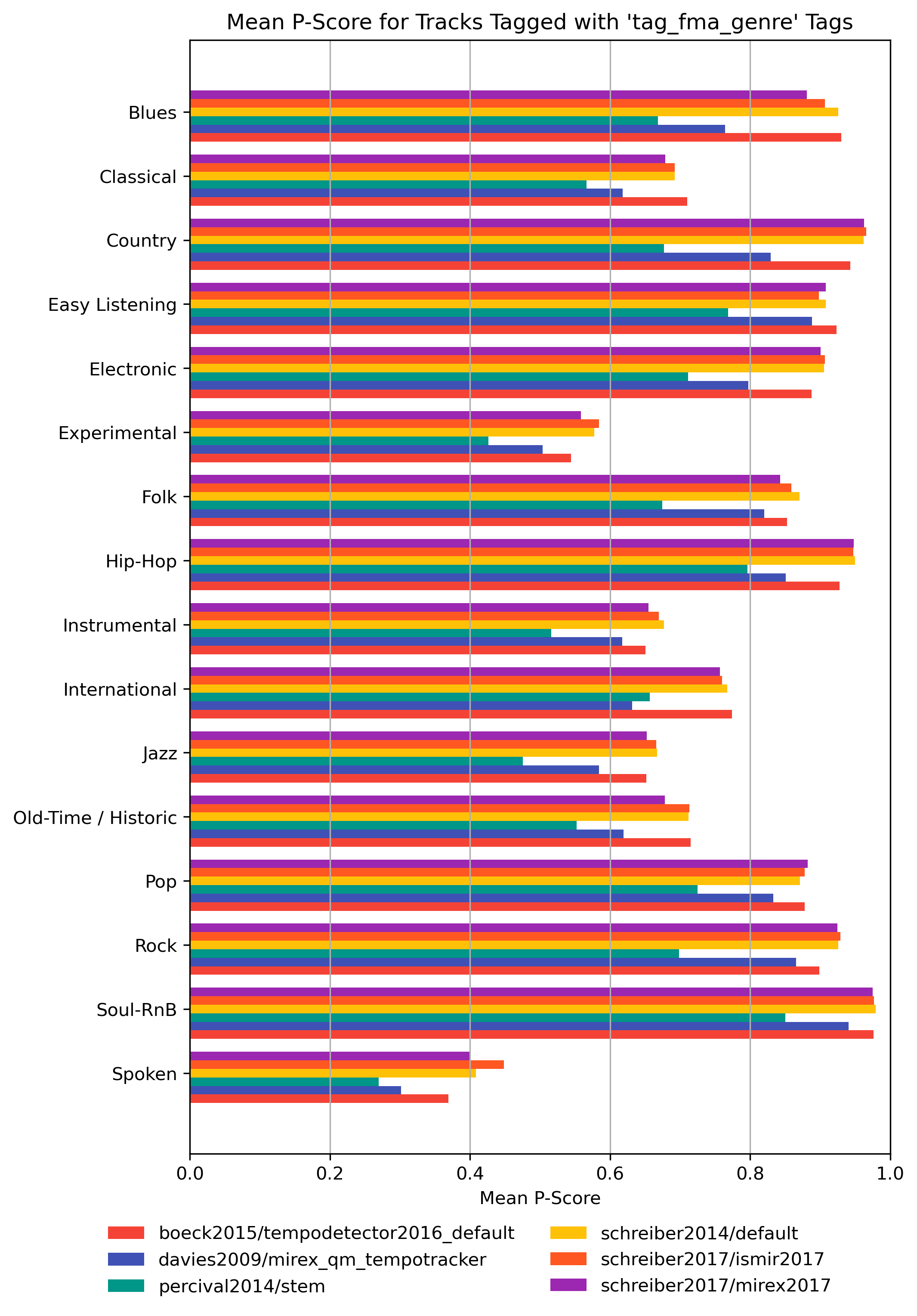
P-Score is defined as the average of two tempi weighted by their perceptual strength, allowing an 8% tolerance for both tempo values [MIREX 2006 Definition].
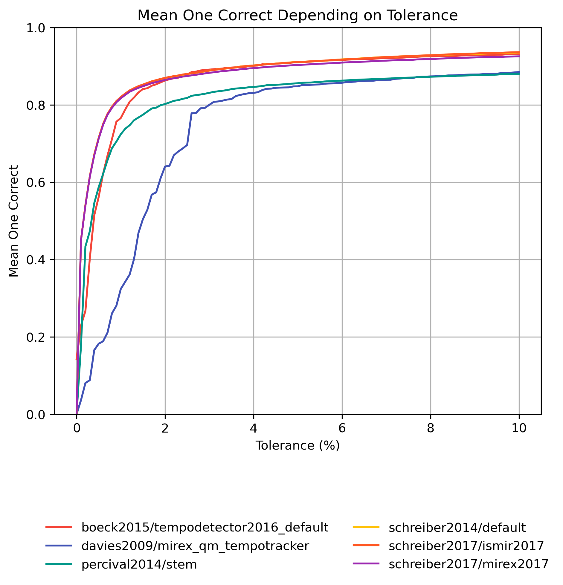
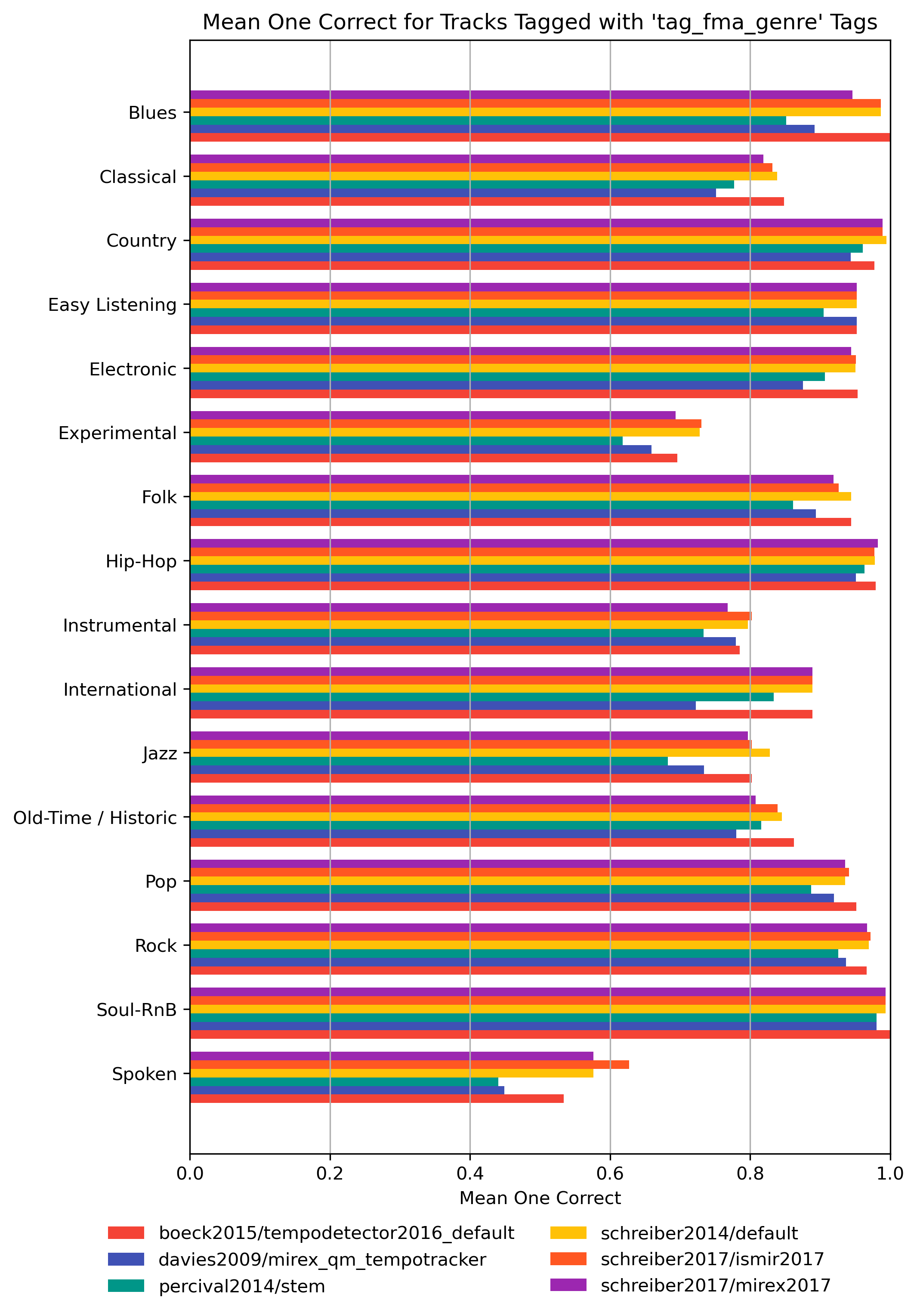
One Correct is the fraction of estimate pairs of which at least one of the two values is equal to a reference value (within an 8% tolerance).
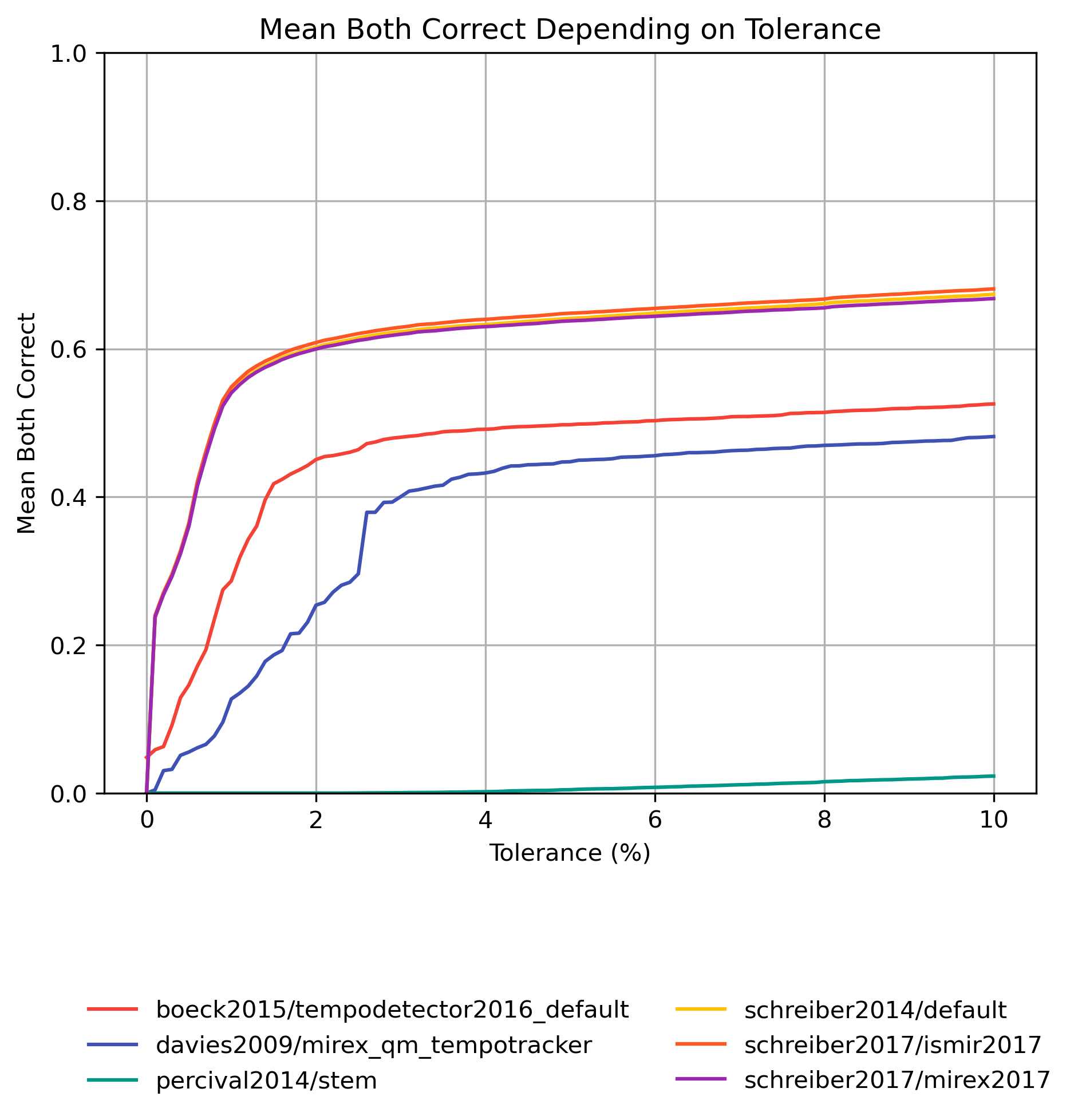
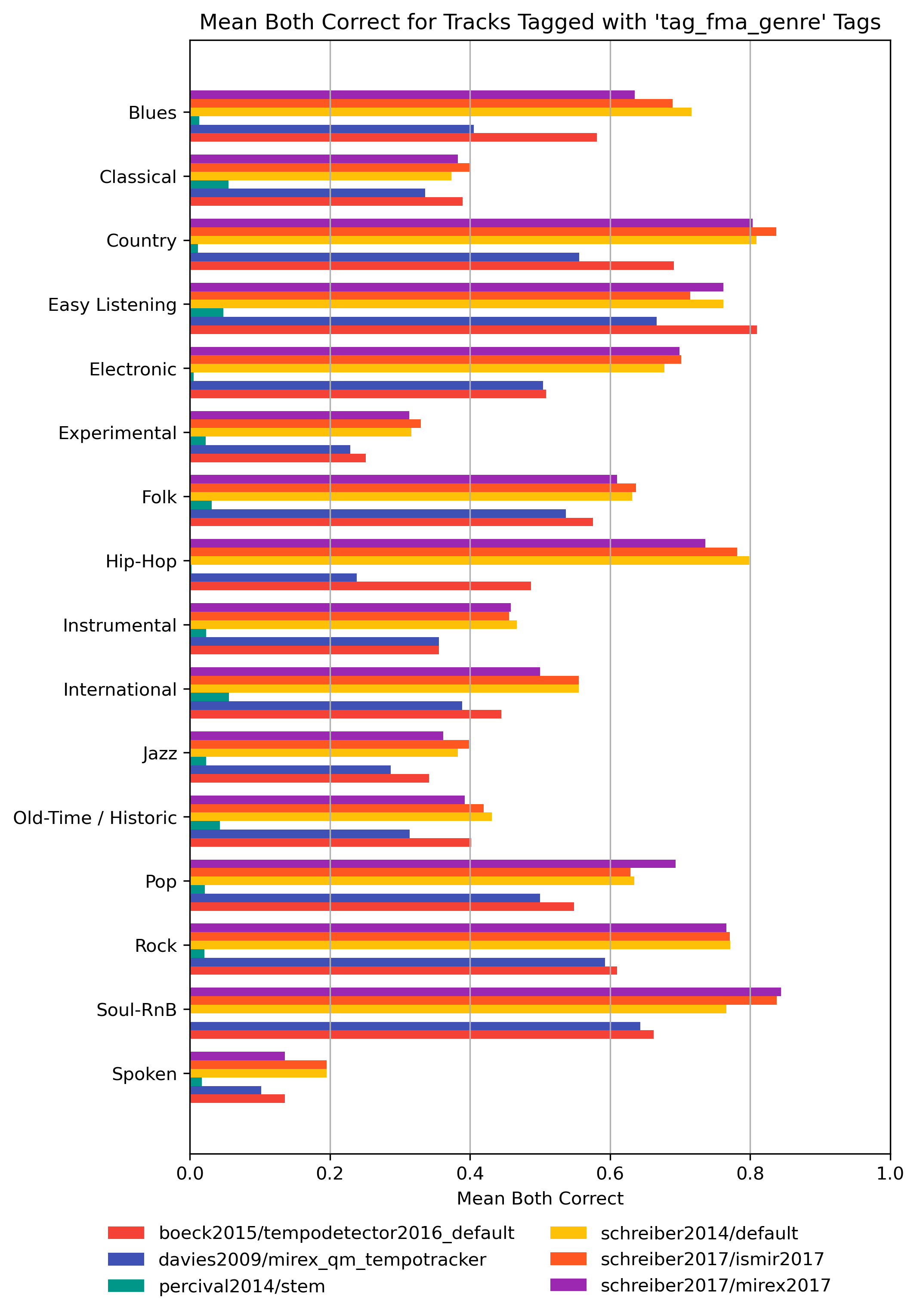
Both Correct is the fraction of estimate pairs of which both values are equal to the reference values (within an 8% tolerance).
See [McKinney2007].
Note: Very few datasets actually have multiple annotations per track along with a salience distributions. References without suitable annotations are not shown.
MIREX Results for schreiber2018/ismir2018
| Estimator | P-Score | One Correct | Both Correct |
|---|---|---|---|
| schreiber2017/ismir2017 | 0.8662 | 0.9284 | 0.6673 |
| schreiber2014/default | 0.8651 | 0.9281 | 0.6611 |
| schreiber2017/mirex2017 | 0.8578 | 0.9185 | 0.6554 |
| boeck2015/tempodetector2016_default | 0.8447 | 0.9254 | 0.5141 |
| davies2009/mirex_qm_tempotracker | 0.7828 | 0.8737 | 0.4697 |
| percival2014/stem | 0.6698 | 0.8728 | 0.0154 |
Table 6: Compared to schreiber2018/ismir2018 with 8.0% tolerance.
Raw data P-Score: CSV JSON LATEX PICKLE
Raw data One Correct: CSV JSON LATEX PICKLE
Raw data Both Correct: CSV JSON LATEX PICKLE
P-Score for schreiber2018/ismir2018
Figure 12: Mean P-Score for estimates compared to version schreiber2018/ismir2018 depending on tolerance.
CSV JSON LATEX PICKLE SVG PDF PNG
One Correct for schreiber2018/ismir2018
Figure 13: Mean One Correct for estimates compared to version schreiber2018/ismir2018 depending on tolerance.
CSV JSON LATEX PICKLE SVG PDF PNG
Both Correct for schreiber2018/ismir2018
Figure 14: Mean Both Correct for estimates compared to version schreiber2018/ismir2018 depending on tolerance.
CSV JSON LATEX PICKLE SVG PDF PNG
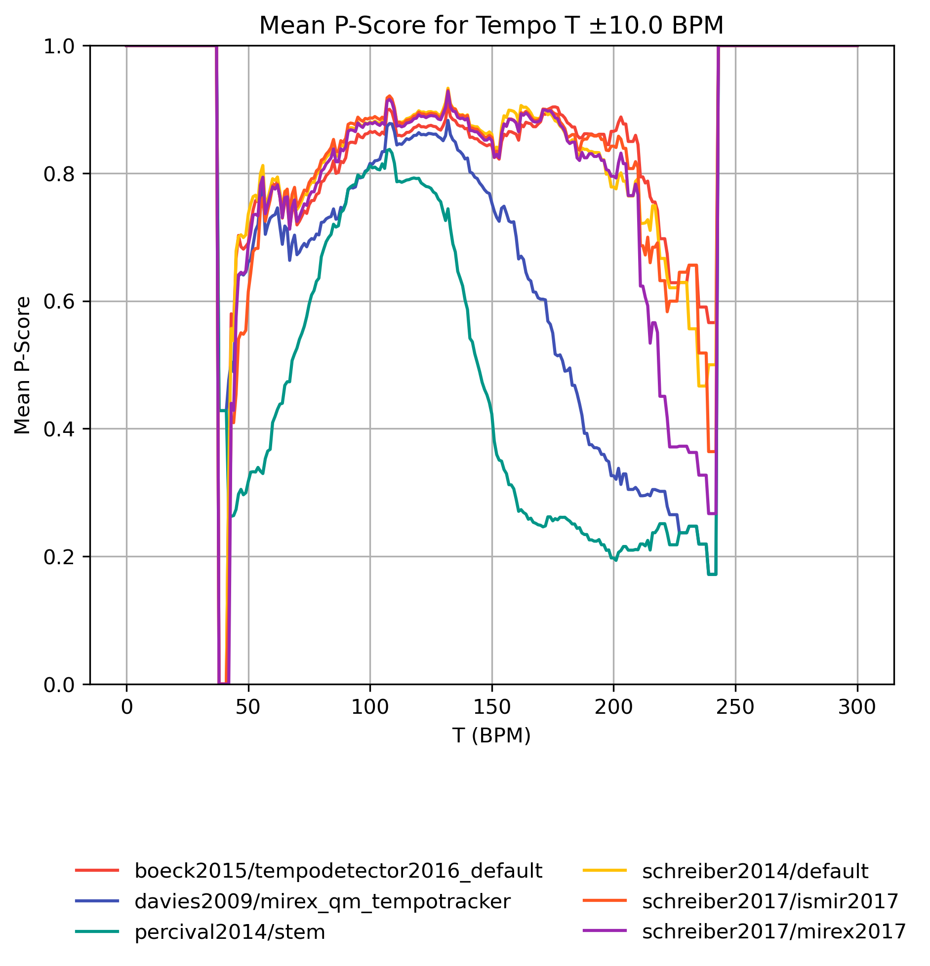
P-Score on Tempo-Subsets
How well does an estimator perform, when only taking a subset of the reference annotations into account? The graphs show mean P-Score for reference subsets with tempi in [T-10,T+10] BPM. Note that the graphs do not show confidence intervals and that some values may be based on very few estimates.
P-Score on Tempo-Subsets for schreiber2018/ismir2018
Figure 15: Mean P-Score for estimates compared to version schreiber2018/ismir2018 for tempo intervals around T.
CSV JSON LATEX PICKLE SVG PDF PNG
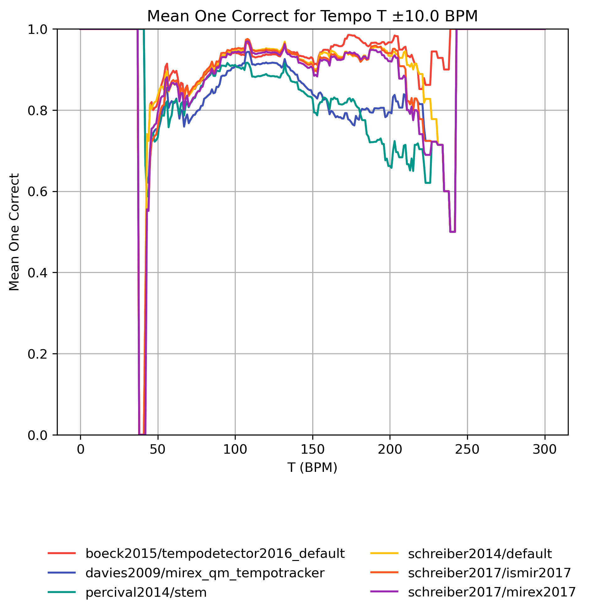
One Correct on Tempo-Subsets
How well does an estimator perform, when only taking a subset of the reference annotations into account? The graphs show mean One Correct for reference subsets with tempi in [T-10,T+10] BPM. Note that the graphs do not show confidence intervals and that some values may be based on very few estimates.
One Correct on Tempo-Subsets for schreiber2018/ismir2018
Figure 16: Mean One Correct for estimates compared to version schreiber2018/ismir2018 for tempo intervals around T.
CSV JSON LATEX PICKLE SVG PDF PNG
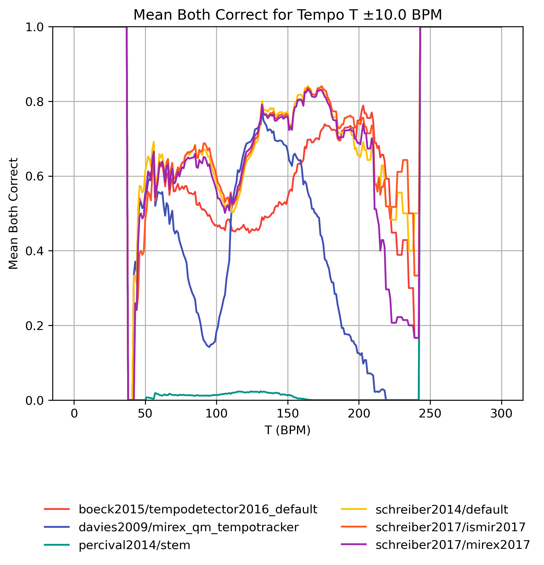
Both Correct on Tempo-Subsets
How well does an estimator perform, when only taking a subset of the reference annotations into account? The graphs show mean Both Correct for reference subsets with tempi in [T-10,T+10] BPM. Note that the graphs do not show confidence intervals and that some values may be based on very few estimates.
Both Correct on Tempo-Subsets for schreiber2018/ismir2018
Figure 17: Mean Both Correct for estimates compared to version schreiber2018/ismir2018 for tempo intervals around T.
CSV JSON LATEX PICKLE SVG PDF PNG
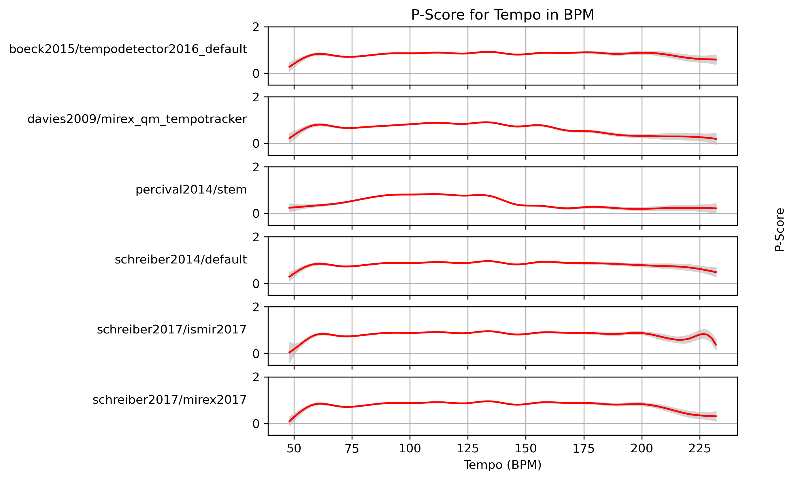
Estimated P-Score for Tempo
When fitting a generalized additive model (GAM) to P-Score-values and a ground truth, what P-Score can we expect with confidence?
Estimated P-Score for Tempo for schreiber2018/ismir2018
Predictions of GAMs trained on P-Score for estimates for reference schreiber2018/ismir2018.
Figure 18: P-Score predictions of a generalized additive model (GAM) fit to P-Score results for schreiber2018/ismir2018. The 95% confidence interval around the prediction is shaded in gray.
CSV JSON LATEX PICKLE SVG PDF PNG
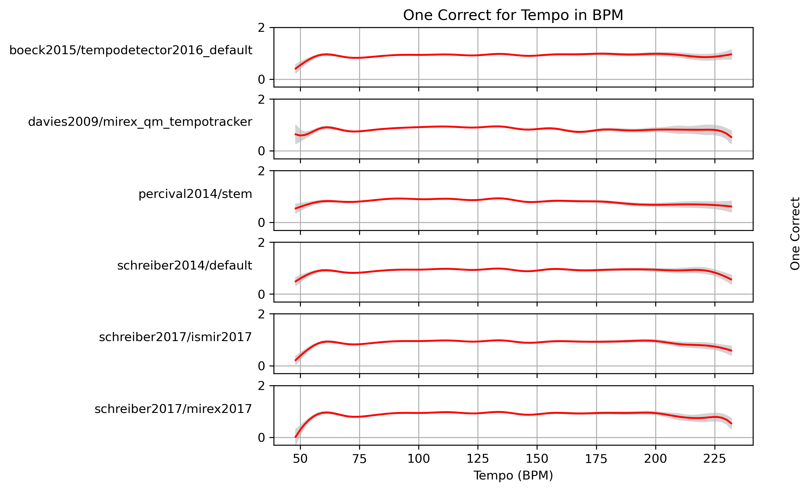
Estimated One Correct for Tempo
When fitting a generalized additive model (GAM) to One Correct-values and a ground truth, what One Correct can we expect with confidence?
Estimated One Correct for Tempo for schreiber2018/ismir2018
Predictions of GAMs trained on One Correct for estimates for reference schreiber2018/ismir2018.
Figure 19: One Correct predictions of a generalized additive model (GAM) fit to One Correct results for schreiber2018/ismir2018. The 95% confidence interval around the prediction is shaded in gray.
CSV JSON LATEX PICKLE SVG PDF PNG
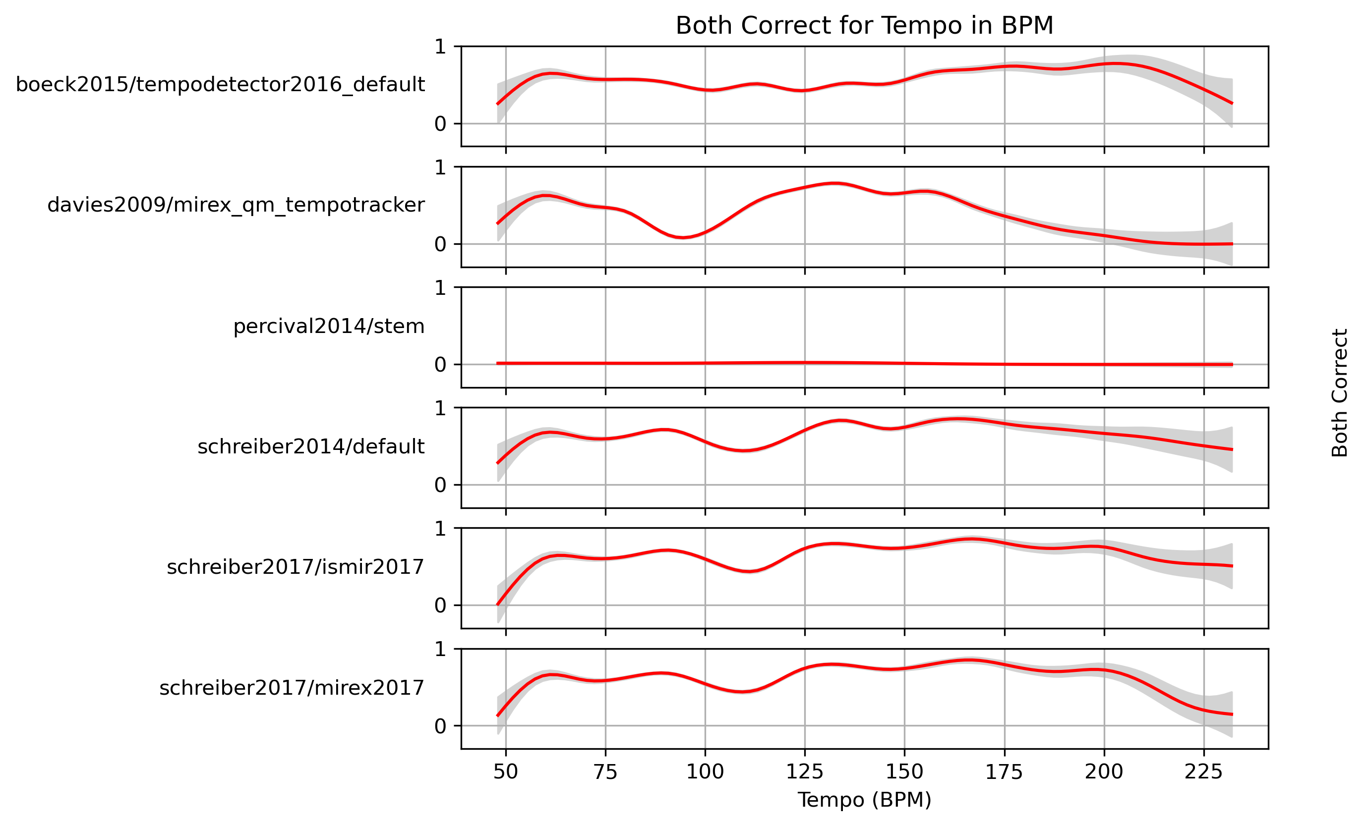
Estimated Both Correct for Tempo
When fitting a generalized additive model (GAM) to Both Correct-values and a ground truth, what Both Correct can we expect with confidence?
Estimated Both Correct for Tempo for schreiber2018/ismir2018
Predictions of GAMs trained on Both Correct for estimates for reference schreiber2018/ismir2018.
Figure 20: Both Correct predictions of a generalized additive model (GAM) fit to Both Correct results for schreiber2018/ismir2018. The 95% confidence interval around the prediction is shaded in gray.
CSV JSON LATEX PICKLE SVG PDF PNG
P-Score for ‘tag_fma_genre’ Tags
How well does an estimator perform, when only taking tracks into account that are tagged with some kind of label? Note that some values may be based on very few estimates.
P-Score for ‘tag_fma_genre’ Tags for schreiber2018/ismir2018
Figure 21: Mean P-Score of estimates compared to version schreiber2018/ismir2018 depending on tag from namespace ‘tag_fma_genre’.
CSV JSON LATEX PICKLE SVG PDF PNG
One Correct for ‘tag_fma_genre’ Tags
How well does an estimator perform, when only taking tracks into account that are tagged with some kind of label? Note that some values may be based on very few estimates.
One Correct for ‘tag_fma_genre’ Tags for schreiber2018/ismir2018
Figure 22: Mean One Correct of estimates compared to version schreiber2018/ismir2018 depending on tag from namespace ‘tag_fma_genre’.
CSV JSON LATEX PICKLE SVG PDF PNG
Both Correct for ‘tag_fma_genre’ Tags
How well does an estimator perform, when only taking tracks into account that are tagged with some kind of label? Note that some values may be based on very few estimates.
Both Correct for ‘tag_fma_genre’ Tags for schreiber2018/ismir2018
Figure 23: Mean Both Correct of estimates compared to version schreiber2018/ismir2018 depending on tag from namespace ‘tag_fma_genre’.
CSV JSON LATEX PICKLE SVG PDF PNG
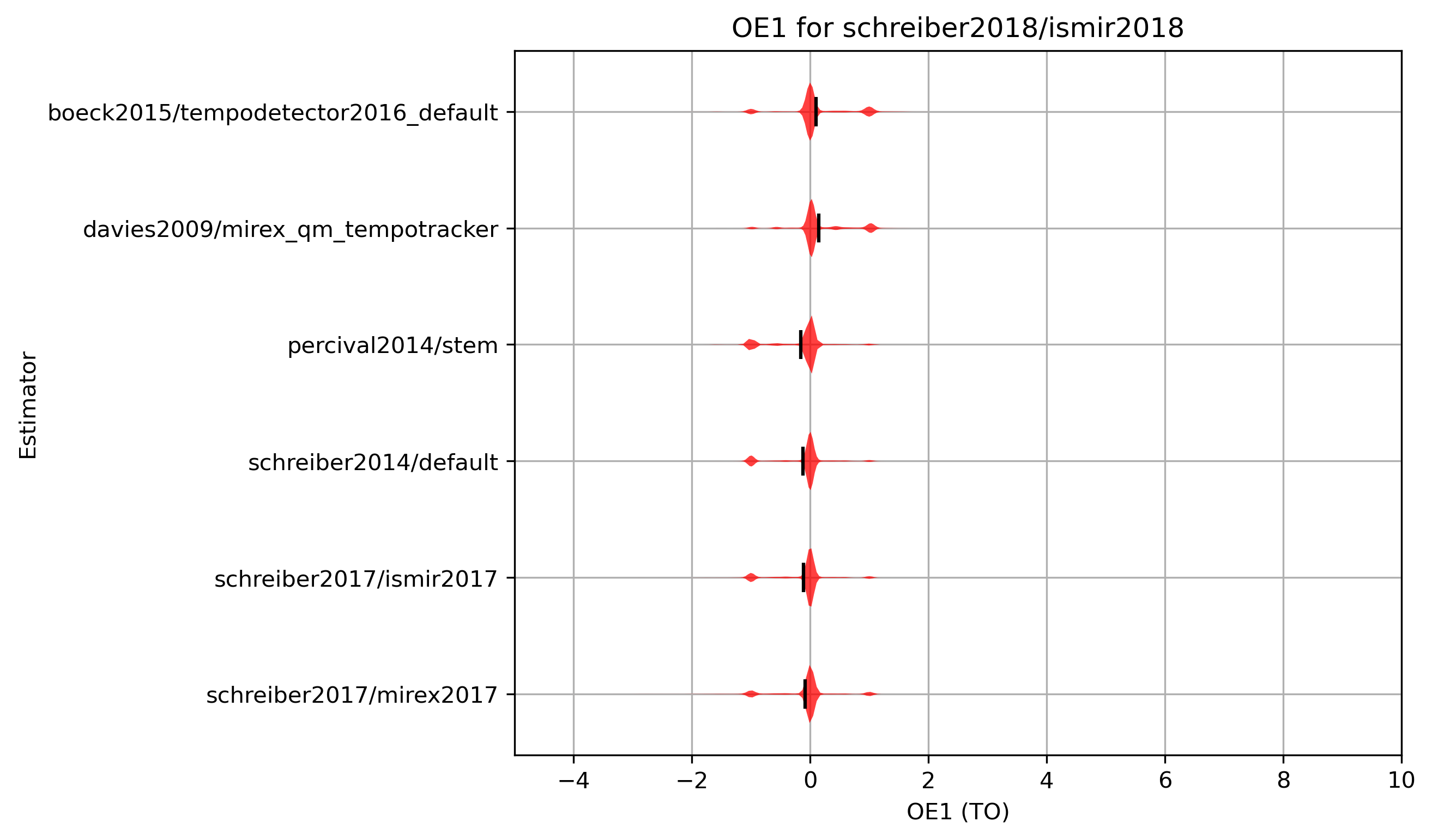
OE1 and OE2
OE1 is defined as octave error between an estimate E and a reference value R.This means that the most common errors—by a factor of 2 or ½—have the same magnitude, namely 1: OE2(E) = log2(E/R).
OE2 is the signed OE1 corresponding to the minimum absolute OE1 allowing the octaveerrors 2, 3, 1/2, and 1/3: OE2(E) = arg minx(|x|) with x ∈ {OE1(E), OE1(2E), OE1(3E), OE1(½E), OE1(⅓E)}
Mean OE1/OE2 Results for schreiber2018/ismir2018
| Estimator | OE1_MEAN | OE1_STDEV | OE2_MEAN | OE2_STDEV |
|---|---|---|---|---|
| schreiber2014/default | -0.1188 | 0.4184 | -0.0022 | 0.1180 |
| schreiber2017/ismir2017 | -0.1117 | 0.4250 | -0.0025 | 0.1216 |
| davies2009/mirex_qm_tempotracker | 0.1484 | 0.4325 | 0.0349 | 0.1455 |
| percival2014/stem | -0.1566 | 0.4467 | 0.0112 | 0.1465 |
| schreiber2017/mirex2017 | -0.0898 | 0.4800 | -0.0048 | 0.1305 |
| boeck2015/tempodetector2016_default | 0.0975 | 0.4947 | -0.0009 | 0.1124 |
Table 7: Mean OE1/OE2 for estimates compared to version schreiber2018/ismir2018 ordered by standard deviation.
Raw data OE1: CSV JSON LATEX PICKLE
Raw data OE2: CSV JSON LATEX PICKLE
OE1 distribution for schreiber2018/ismir2018
Figure 24: OE1 for estimates compared to version schreiber2018/ismir2018. Shown are the mean OE1 and an empirical distribution of the sample, using kernel density estimation (KDE).
CSV JSON LATEX PICKLE SVG PDF PNG
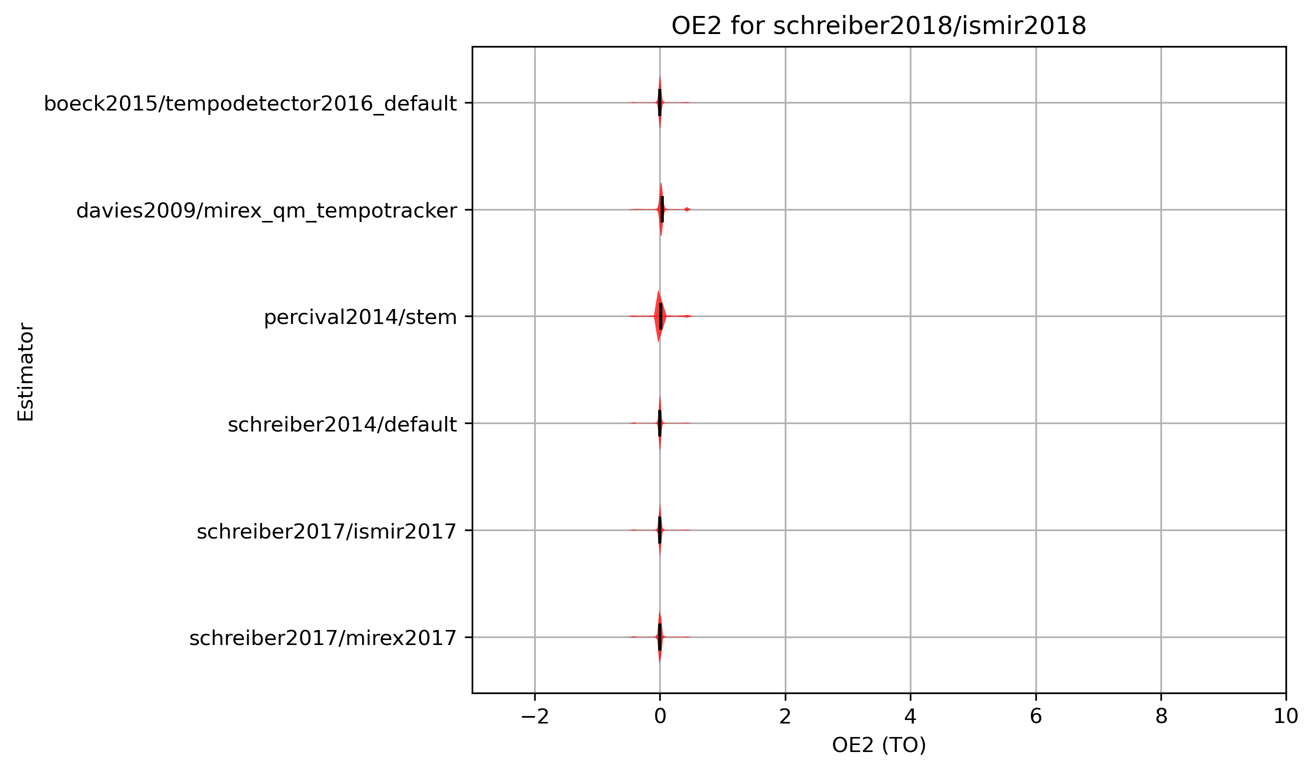
OE2 distribution for schreiber2018/ismir2018
Figure 25: OE2 for estimates compared to version schreiber2018/ismir2018. Shown are the mean OE2 and an empirical distribution of the sample, using kernel density estimation (KDE).
CSV JSON LATEX PICKLE SVG PDF PNG
Significance of Differences
| Estimator | boeck2015/tempodetector2016_default | davies2009/mirex_qm_tempotracker | percival2014/stem | schreiber2014/default | schreiber2017/ismir2017 | schreiber2017/mirex2017 |
|---|---|---|---|---|---|---|
| boeck2015/tempodetector2016_default | 1.0000 | 0.0000 | 0.0000 | 0.0000 | 0.0000 | 0.0000 |
| davies2009/mirex_qm_tempotracker | 0.0000 | 1.0000 | 0.0000 | 0.0000 | 0.0000 | 0.0000 |
| percival2014/stem | 0.0000 | 0.0000 | 1.0000 | 0.0000 | 0.0000 | 0.0000 |
| schreiber2014/default | 0.0000 | 0.0000 | 0.0000 | 1.0000 | 0.0076 | 0.0000 |
| schreiber2017/ismir2017 | 0.0000 | 0.0000 | 0.0000 | 0.0076 | 1.0000 | 0.0000 |
| schreiber2017/mirex2017 | 0.0000 | 0.0000 | 0.0000 | 0.0000 | 0.0000 | 1.0000 |
Table 8: Paired t-test p-values, using reference annotations schreiber2018/ismir2018 as groundtruth with OE1. H0: the true mean difference between paired samples is zero. If p<=ɑ, reject H0, i.e. we have a significant difference between estimates from the two algorithms. In the table, p-values<0.05 are set in bold.
| Estimator | boeck2015/tempodetector2016_default | davies2009/mirex_qm_tempotracker | percival2014/stem | schreiber2014/default | schreiber2017/ismir2017 | schreiber2017/mirex2017 |
|---|---|---|---|---|---|---|
| boeck2015/tempodetector2016_default | 1.0000 | 0.0000 | 0.0000 | 0.1656 | 0.0908 | 0.0001 |
| davies2009/mirex_qm_tempotracker | 0.0000 | 1.0000 | 0.0000 | 0.0000 | 0.0000 | 0.0000 |
| percival2014/stem | 0.0000 | 0.0000 | 1.0000 | 0.0000 | 0.0000 | 0.0000 |
| schreiber2014/default | 0.1656 | 0.0000 | 0.0000 | 1.0000 | 0.7343 | 0.0032 |
| schreiber2017/ismir2017 | 0.0908 | 0.0000 | 0.0000 | 0.7343 | 1.0000 | 0.0000 |
| schreiber2017/mirex2017 | 0.0001 | 0.0000 | 0.0000 | 0.0032 | 0.0000 | 1.0000 |
Table 9: Paired t-test p-values, using reference annotations schreiber2018/ismir2018 as groundtruth with OE2. H0: the true mean difference between paired samples is zero. If p<=ɑ, reject H0, i.e. we have a significant difference between estimates from the two algorithms. In the table, p-values<0.05 are set in bold.
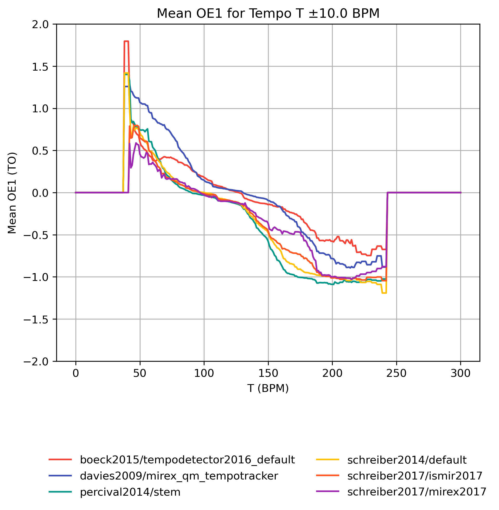
OE1 on Tempo-Subsets
How well does an estimator perform, when only taking a subset of the reference annotations into account? The graphs show mean OE1 for reference subsets with tempi in [T-10,T+10] BPM. Note that the graphs do not show confidence intervals and that some values may be based on very few estimates.
OE1 on Tempo-Subsets for schreiber2018/ismir2018
Figure 26: Mean OE1 for estimates compared to version schreiber2018/ismir2018 for tempo intervals around T.
CSV JSON LATEX PICKLE SVG PDF PNG
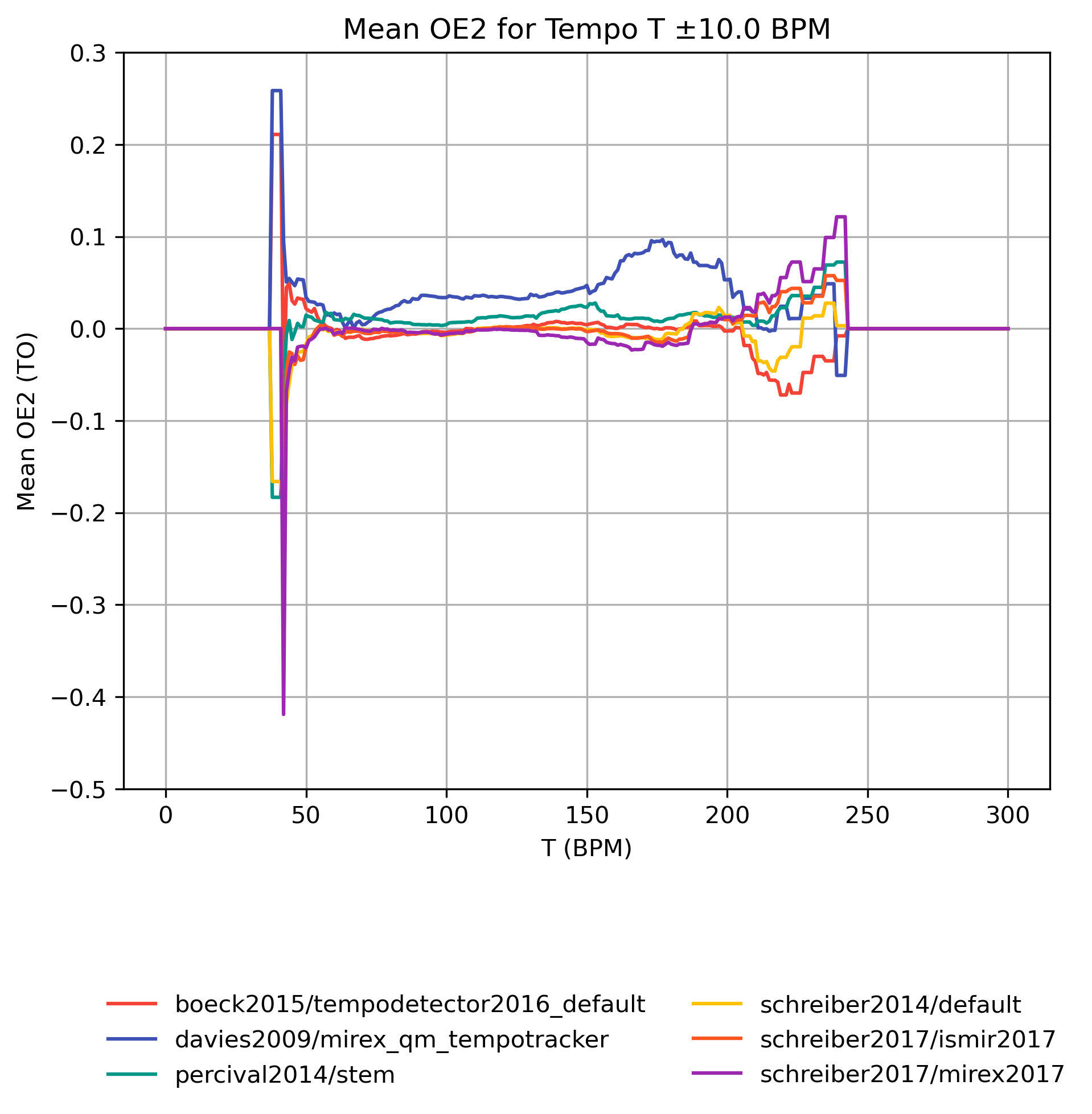
OE2 on Tempo-Subsets
How well does an estimator perform, when only taking a subset of the reference annotations into account? The graphs show mean OE2 for reference subsets with tempi in [T-10,T+10] BPM. Note that the graphs do not show confidence intervals and that some values may be based on very few estimates.
OE2 on Tempo-Subsets for schreiber2018/ismir2018
Figure 27: Mean OE2 for estimates compared to version schreiber2018/ismir2018 for tempo intervals around T.
CSV JSON LATEX PICKLE SVG PDF PNG
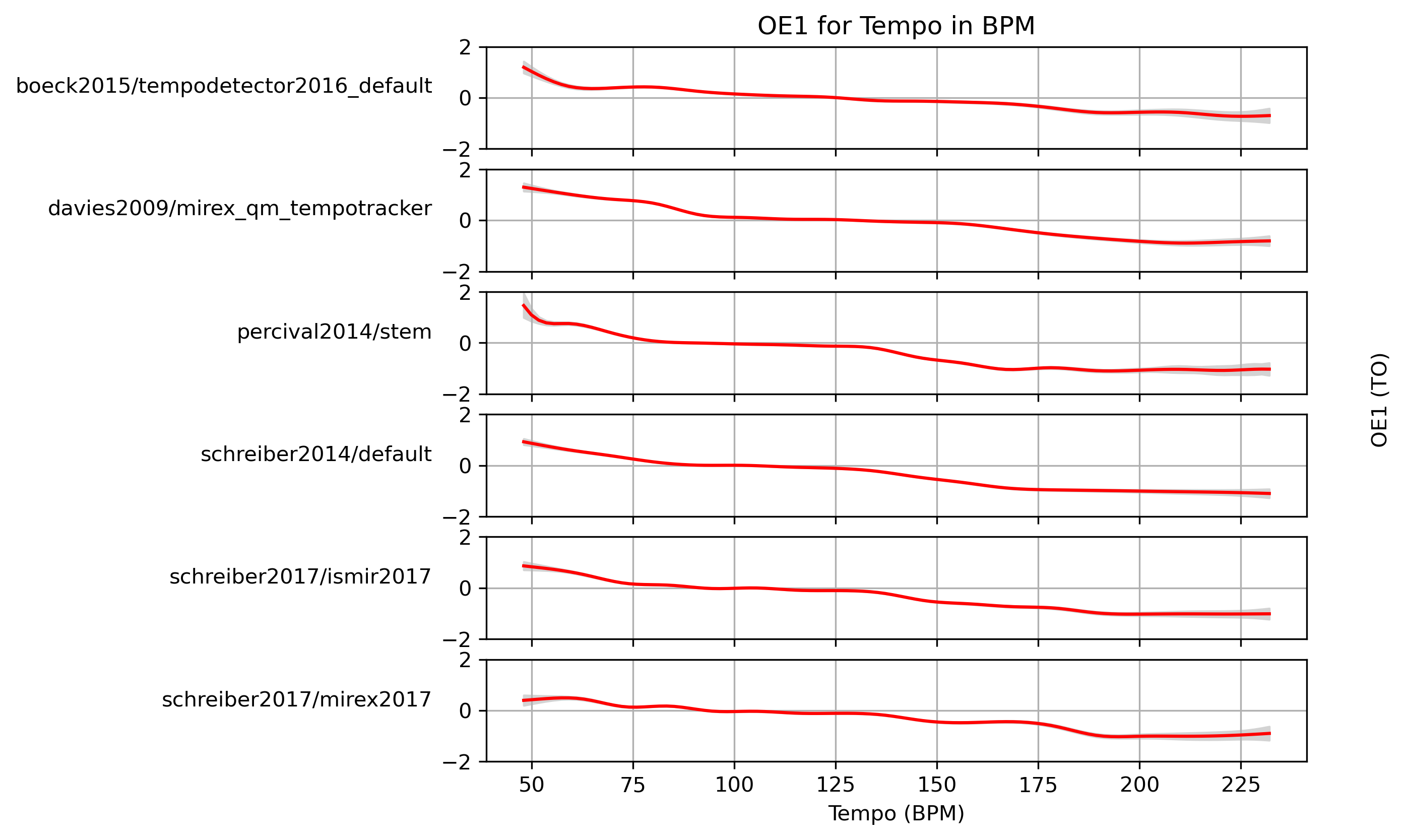
Estimated OE1 for Tempo
When fitting a generalized additive model (GAM) to OE1-values and a ground truth, what OE1 can we expect with confidence?
Estimated OE1 for Tempo for schreiber2018/ismir2018
Predictions of GAMs trained on OE1 for estimates for reference schreiber2018/ismir2018.
Figure 28: OE1 predictions of a generalized additive model (GAM) fit to OE1 results for schreiber2018/ismir2018. The 95% confidence interval around the prediction is shaded in gray.
CSV JSON LATEX PICKLE SVG PDF PNG
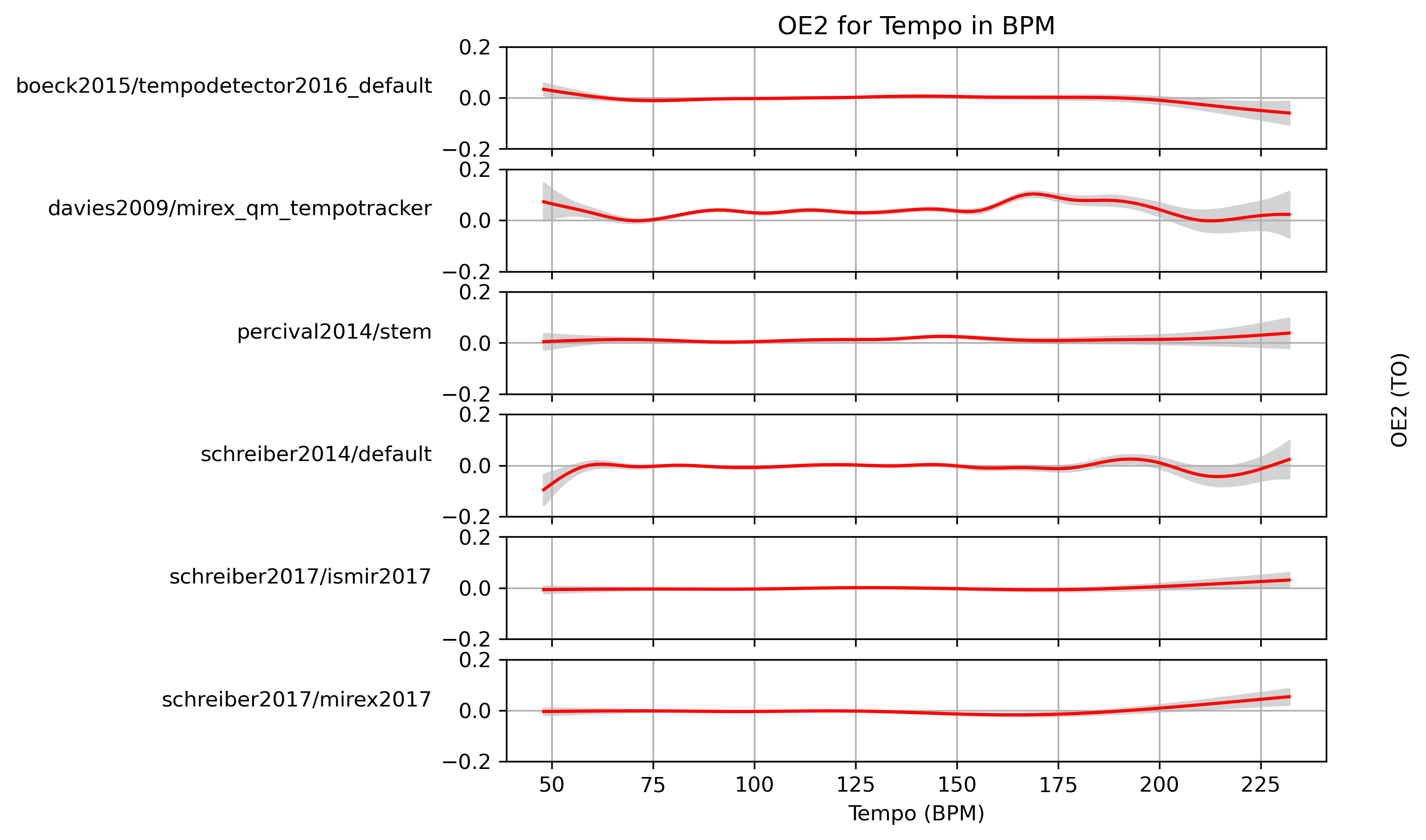
Estimated OE2 for Tempo
When fitting a generalized additive model (GAM) to OE2-values and a ground truth, what OE2 can we expect with confidence?
Estimated OE2 for Tempo for schreiber2018/ismir2018
Predictions of GAMs trained on OE2 for estimates for reference schreiber2018/ismir2018.
Figure 29: OE2 predictions of a generalized additive model (GAM) fit to OE2 results for schreiber2018/ismir2018. The 95% confidence interval around the prediction is shaded in gray.
CSV JSON LATEX PICKLE SVG PDF PNG
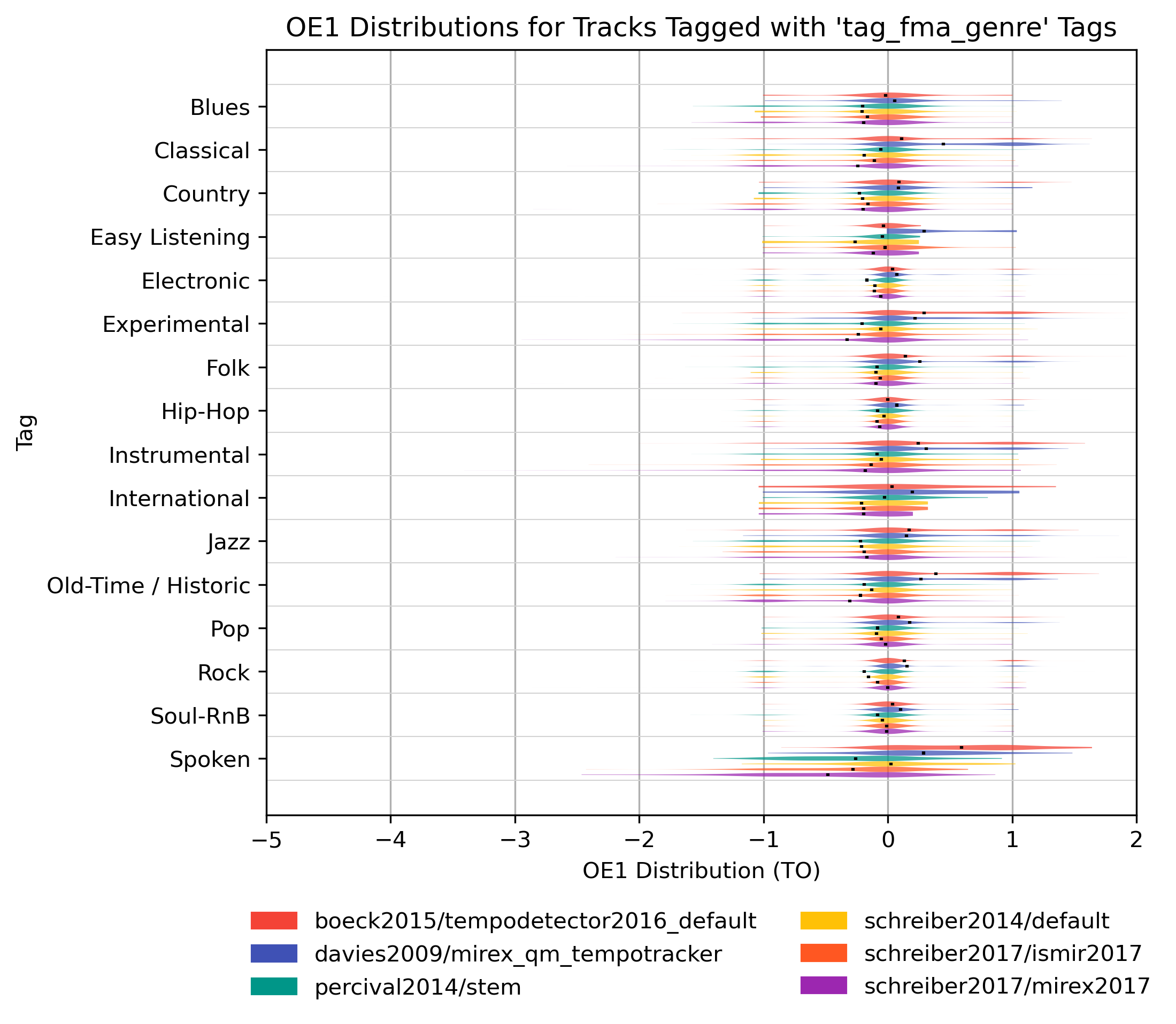
OE1 for ‘tag_fma_genre’ Tags
How well does an estimator perform, when only taking tracks into account that are tagged with some kind of label? Note that some values may be based on very few estimates.
OE1 for ‘tag_fma_genre’ Tags for schreiber2018/ismir2018
Figure 30: OE1 of estimates compared to version schreiber2018/ismir2018 depending on tag from namespace ‘tag_fma_genre’.
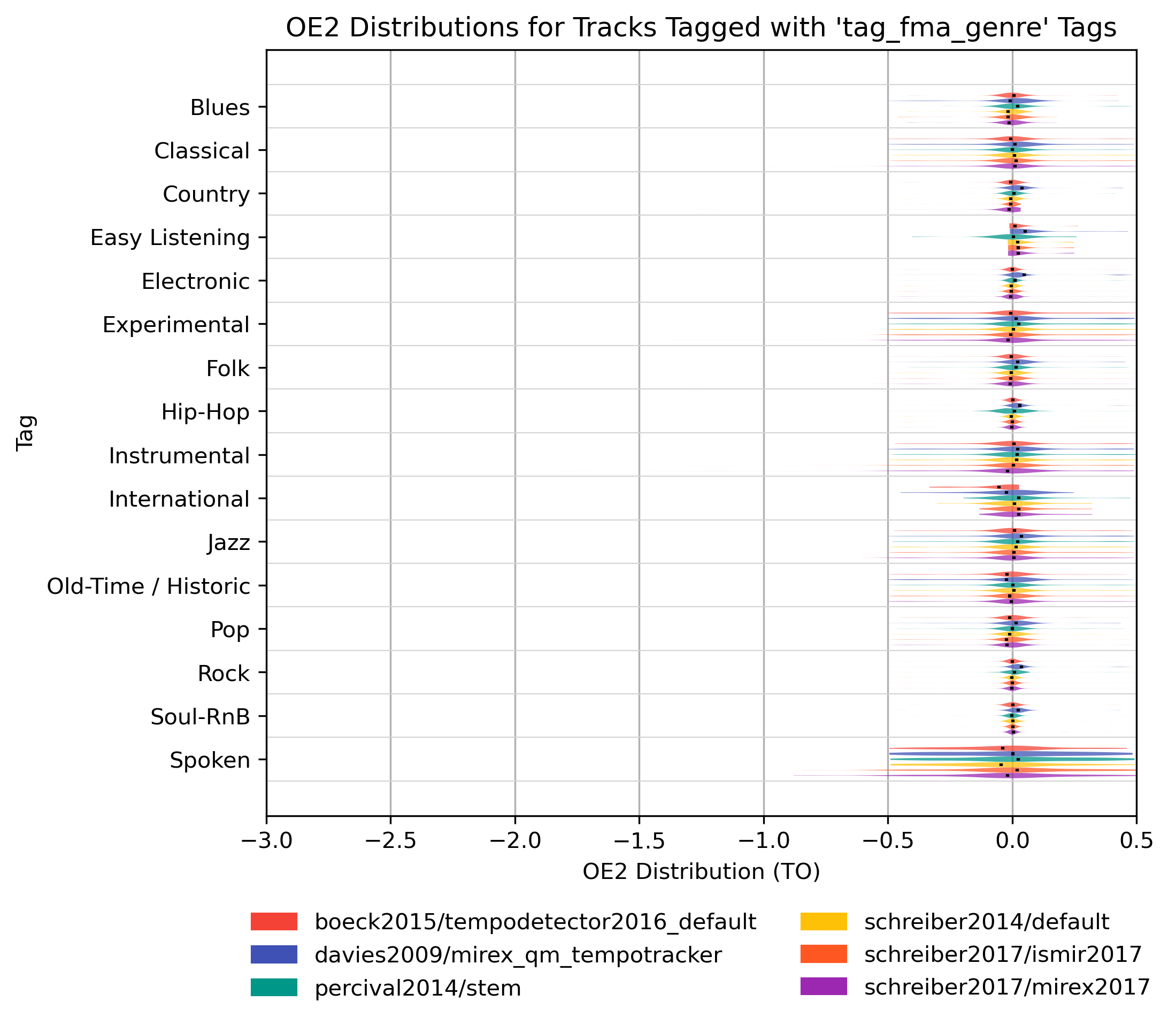
OE2 for ‘tag_fma_genre’ Tags
How well does an estimator perform, when only taking tracks into account that are tagged with some kind of label? Note that some values may be based on very few estimates.
OE2 for ‘tag_fma_genre’ Tags for schreiber2018/ismir2018
Figure 31: OE2 of estimates compared to version schreiber2018/ismir2018 depending on tag from namespace ‘tag_fma_genre’.
AOE1 and AOE2
AOE1 is defined as absolute octave error between an estimate and a reference value: AOE1(E) = |log2(E/R)|.
AOE2 is the minimum of AOE1 allowing the octave errors 2, 3, 1/2, and 1/3: AOE2(E) = min(AOE1(E), AOE1(2E), AOE1(3E), AOE1(½E), AOE1(⅓E)).
Mean AOE1/AOE2 Results for schreiber2018/ismir2018
| Estimator | AOE1_MEAN | AOE1_STDEV | AOE2_MEAN | AOE2_STDEV |
|---|---|---|---|---|
| schreiber2017/ismir2017 | 0.2121 | 0.3849 | 0.0454 | 0.1128 |
| schreiber2014/default | 0.2174 | 0.3768 | 0.0443 | 0.1093 |
| schreiber2017/mirex2017 | 0.2348 | 0.4282 | 0.0461 | 0.1222 |
| percival2014/stem | 0.2409 | 0.4075 | 0.0485 | 0.1387 |
| davies2009/mirex_qm_tempotracker | 0.2520 | 0.3815 | 0.0766 | 0.1285 |
| boeck2015/tempodetector2016_default | 0.2703 | 0.4257 | 0.0444 | 0.1033 |
Table 10: Mean AOE1/AOE2 for estimates compared to version schreiber2018/ismir2018 ordered by mean.
Raw data AOE1: CSV JSON LATEX PICKLE
Raw data AOE2: CSV JSON LATEX PICKLE
AOE1 distribution for schreiber2018/ismir2018
Figure 32: AOE1 for estimates compared to version schreiber2018/ismir2018. Shown are the mean AOE1 and an empirical distribution of the sample, using kernel density estimation (KDE).
CSV JSON LATEX PICKLE SVG PDF PNG
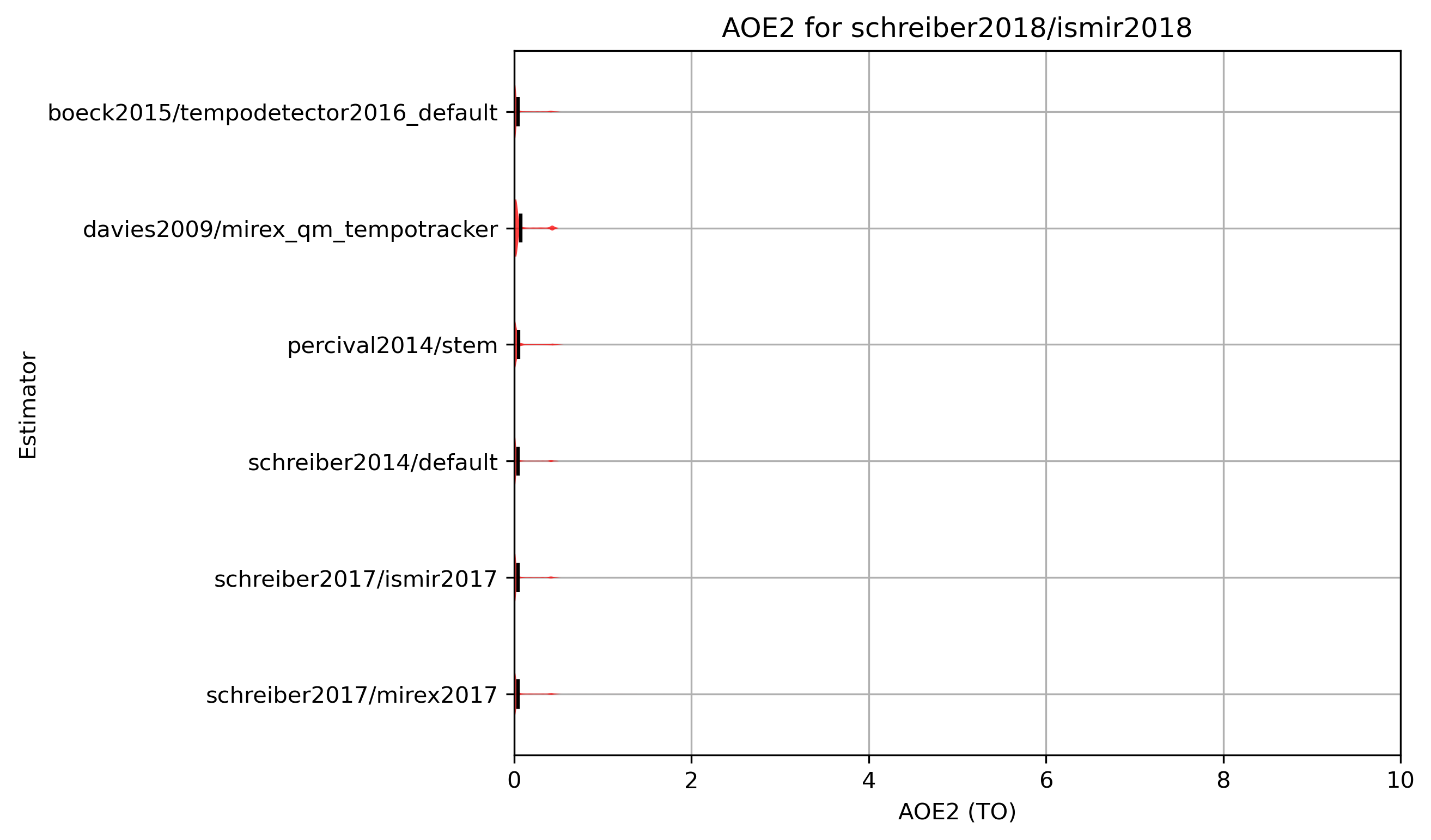
AOE2 distribution for schreiber2018/ismir2018
Figure 33: AOE2 for estimates compared to version schreiber2018/ismir2018. Shown are the mean AOE2 and an empirical distribution of the sample, using kernel density estimation (KDE).
CSV JSON LATEX PICKLE SVG PDF PNG
Significance of Differences
| Estimator | boeck2015/tempodetector2016_default | davies2009/mirex_qm_tempotracker | percival2014/stem | schreiber2014/default | schreiber2017/ismir2017 | schreiber2017/mirex2017 |
|---|---|---|---|---|---|---|
| boeck2015/tempodetector2016_default | 1.0000 | 0.0000 | 0.0000 | 0.0000 | 0.0000 | 0.0000 |
| davies2009/mirex_qm_tempotracker | 0.0000 | 1.0000 | 0.0002 | 0.0000 | 0.0000 | 0.0000 |
| percival2014/stem | 0.0000 | 0.0002 | 1.0000 | 0.0000 | 0.0000 | 0.0476 |
| schreiber2014/default | 0.0000 | 0.0000 | 0.0000 | 1.0000 | 0.0371 | 0.0000 |
| schreiber2017/ismir2017 | 0.0000 | 0.0000 | 0.0000 | 0.0371 | 1.0000 | 0.0000 |
| schreiber2017/mirex2017 | 0.0000 | 0.0000 | 0.0476 | 0.0000 | 0.0000 | 1.0000 |
Table 11: Paired t-test p-values, using reference annotations schreiber2018/ismir2018 as groundtruth with AOE1. H0: the true mean difference between paired samples is zero. If p<=ɑ, reject H0, i.e. we have a significant difference between estimates from the two algorithms. In the table, p-values<0.05 are set in bold.
| Estimator | boeck2015/tempodetector2016_default | davies2009/mirex_qm_tempotracker | percival2014/stem | schreiber2014/default | schreiber2017/ismir2017 | schreiber2017/mirex2017 |
|---|---|---|---|---|---|---|
| boeck2015/tempodetector2016_default | 1.0000 | 0.0000 | 0.0000 | 0.8457 | 0.1198 | 0.0149 |
| davies2009/mirex_qm_tempotracker | 0.0000 | 1.0000 | 0.0000 | 0.0000 | 0.0000 | 0.0000 |
| percival2014/stem | 0.0000 | 0.0000 | 1.0000 | 0.0000 | 0.0005 | 0.0073 |
| schreiber2014/default | 0.8457 | 0.0000 | 0.0000 | 1.0000 | 0.0354 | 0.0028 |
| schreiber2017/ismir2017 | 0.1198 | 0.0000 | 0.0005 | 0.0354 | 1.0000 | 0.0708 |
| schreiber2017/mirex2017 | 0.0149 | 0.0000 | 0.0073 | 0.0028 | 0.0708 | 1.0000 |
Table 12: Paired t-test p-values, using reference annotations schreiber2018/ismir2018 as groundtruth with AOE2. H0: the true mean difference between paired samples is zero. If p<=ɑ, reject H0, i.e. we have a significant difference between estimates from the two algorithms. In the table, p-values<0.05 are set in bold.
AOE1 on Tempo-Subsets
How well does an estimator perform, when only taking a subset of the reference annotations into account? The graphs show mean AOE1 for reference subsets with tempi in [T-10,T+10] BPM. Note that the graphs do not show confidence intervals and that some values may be based on very few estimates.
AOE1 on Tempo-Subsets for schreiber2018/ismir2018
Figure 34: Mean AOE1 for estimates compared to version schreiber2018/ismir2018 for tempo intervals around T.
CSV JSON LATEX PICKLE SVG PDF PNG
AOE2 on Tempo-Subsets
How well does an estimator perform, when only taking a subset of the reference annotations into account? The graphs show mean AOE2 for reference subsets with tempi in [T-10,T+10] BPM. Note that the graphs do not show confidence intervals and that some values may be based on very few estimates.
AOE2 on Tempo-Subsets for schreiber2018/ismir2018
Figure 35: Mean AOE2 for estimates compared to version schreiber2018/ismir2018 for tempo intervals around T.
CSV JSON LATEX PICKLE SVG PDF PNG
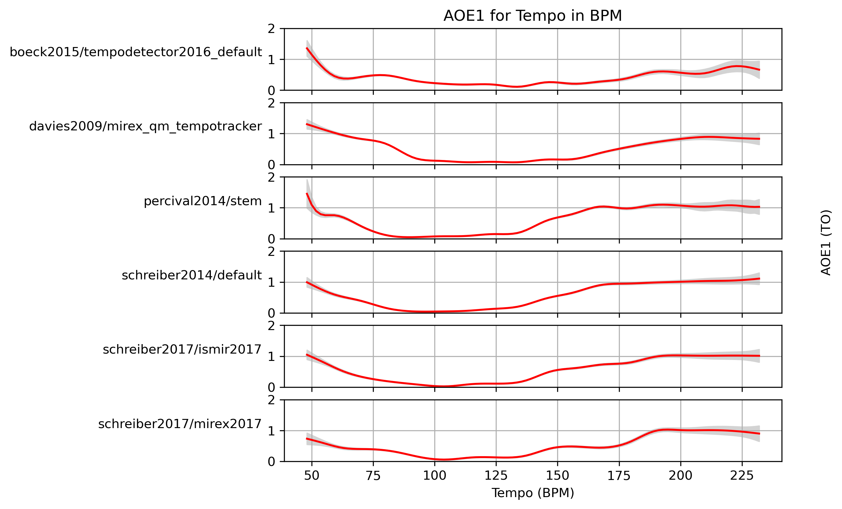
Estimated AOE1 for Tempo
When fitting a generalized additive model (GAM) to AOE1-values and a ground truth, what AOE1 can we expect with confidence?
Estimated AOE1 for Tempo for schreiber2018/ismir2018
Predictions of GAMs trained on AOE1 for estimates for reference schreiber2018/ismir2018.
Figure 36: AOE1 predictions of a generalized additive model (GAM) fit to AOE1 results for schreiber2018/ismir2018. The 95% confidence interval around the prediction is shaded in gray.
CSV JSON LATEX PICKLE SVG PDF PNG
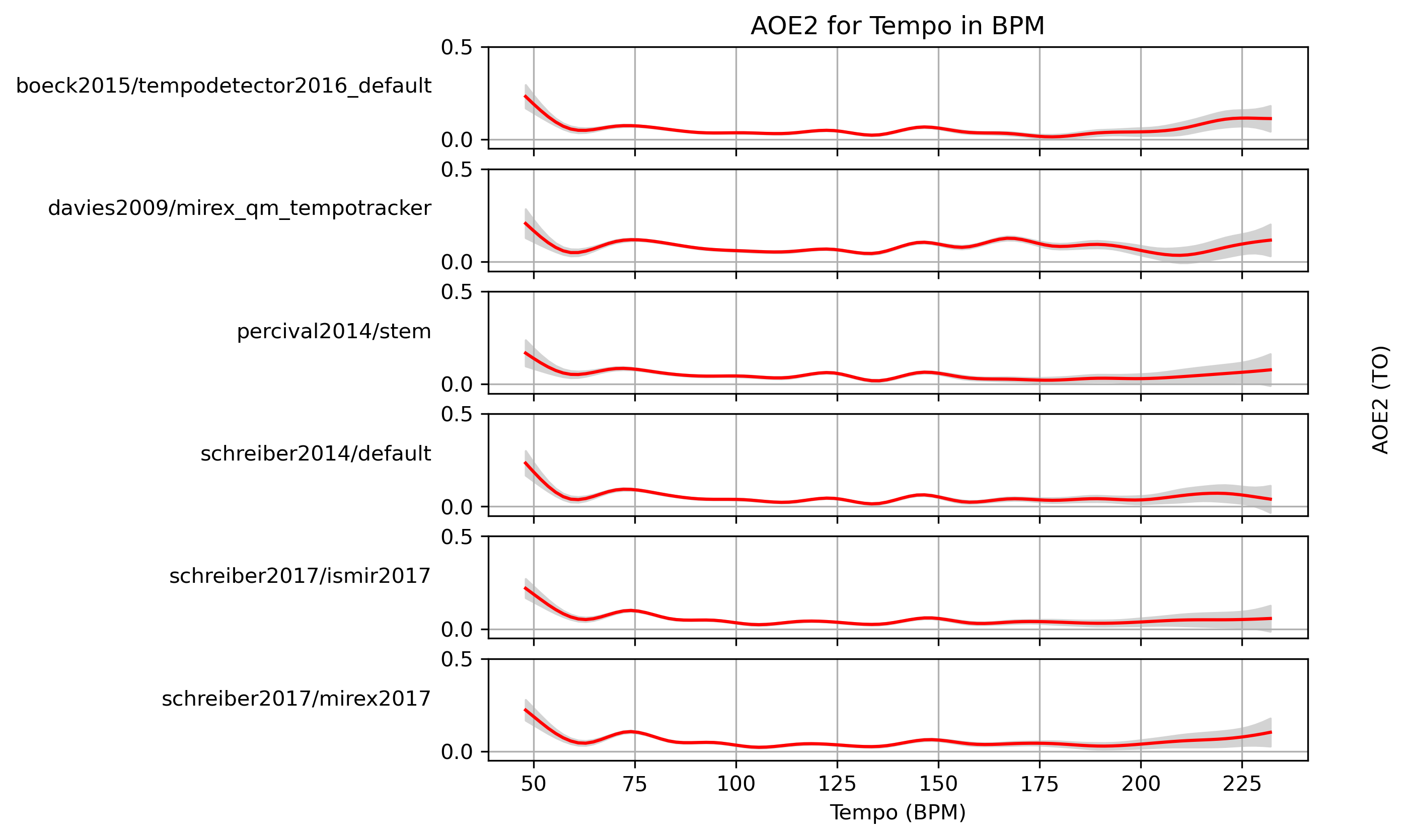
Estimated AOE2 for Tempo
When fitting a generalized additive model (GAM) to AOE2-values and a ground truth, what AOE2 can we expect with confidence?
Estimated AOE2 for Tempo for schreiber2018/ismir2018
Predictions of GAMs trained on AOE2 for estimates for reference schreiber2018/ismir2018.
Figure 37: AOE2 predictions of a generalized additive model (GAM) fit to AOE2 results for schreiber2018/ismir2018. The 95% confidence interval around the prediction is shaded in gray.
CSV JSON LATEX PICKLE SVG PDF PNG
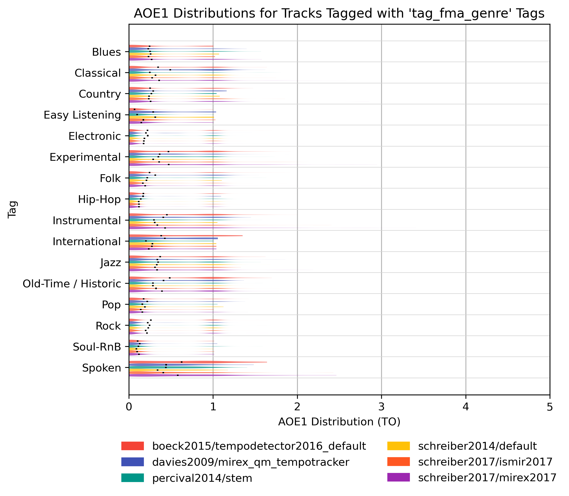
AOE1 for ‘tag_fma_genre’ Tags
How well does an estimator perform, when only taking tracks into account that are tagged with some kind of label? Note that some values may be based on very few estimates.
AOE1 for ‘tag_fma_genre’ Tags for schreiber2018/ismir2018
Figure 38: AOE1 of estimates compared to version schreiber2018/ismir2018 depending on tag from namespace ‘tag_fma_genre’.
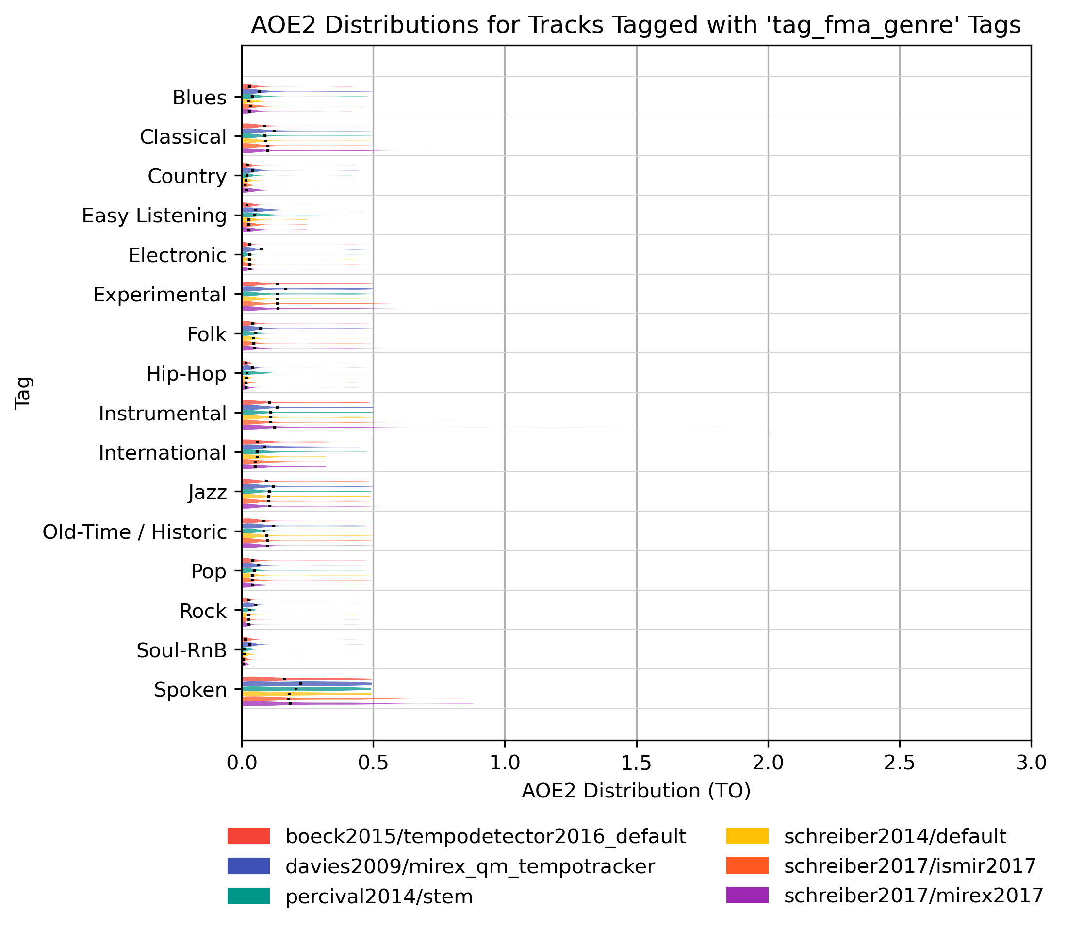
AOE2 for ‘tag_fma_genre’ Tags
How well does an estimator perform, when only taking tracks into account that are tagged with some kind of label? Note that some values may be based on very few estimates.
AOE2 for ‘tag_fma_genre’ Tags for schreiber2018/ismir2018
Figure 39: AOE2 of estimates compared to version schreiber2018/ismir2018 depending on tag from namespace ‘tag_fma_genre’.
Generated by tempo_eval 0.1.1 on 2022-06-29 18:24. Size L.